12.9 Traveling Salesperson Problem

Three doors are shown side-by-side. — **Figure 12.186** Each door on the route of a traveling salesperson can be represented as a vertex on a graph.Each door on the route of a traveling salesperson can be represented as a vertex on a graph. (credit: "Three in a row, Heriot Row" by Jason Mason/Flickr, CC BY 2.1)

Learning Objectives

After completing this section, you should be able to:

Distinguish between brute force algorithms and greedy algorithms.
List all distinct Hamilton cycles of a complete graph.
Apply brute force method to solve traveling salesperson applications.
Apply nearest neighbor method to solve traveling salesperson applications.

We looked at Hamilton cycles and paths in the previous sections Hamilton Cycles and Hamilton Paths. In this section, we will analyze Hamilton cycles in complete weighted graphs to find the shortest route to visit a number of locations and return to the starting point. Besides the many routing applications in which we need the shortest distance, there are also applications in which we search for the route that is least expensive or takes the least time. Here are a few less common applications that you can read about on a website set up by the mathematics department at the University of Waterloo in Ontario, Canada:

Design of fiber optic networks
Minimizing fuel expenses for repositioning satellites
Development of semi-conductors for microchips
A technique for mapping mammalian chromosomes in genome sequencing

Before we look at approaches to solving applications like these, let's discuss the two types of algorithms we will use.

Brute Force and Greedy Algorithms

An algorithm is a sequence of steps that can be used to solve a particular problem. We have solved many problems in this chapter, and the procedures that we used were different types of algorithms. In this section, we will use two common types of algorithms, a brute force algorithm and a greedy algorithm. A brute force algorithm begins by listing every possible solution and applying each one until the best solution is found. A greedy algorithm approaches a problem in stages, making the apparent best choice at each stage, then linking the choices together into an overall solution which may or may not be the best solution.

To understand the difference between these two algorithms, consider the tree diagram in Figure 12.187. Suppose we want to find the path from left to right with the largest total sum. For example, branch A in the tree diagram has a sum of $10 + 2 + 11 + 13 = 36$ .

A graph has 15 vertices. The vertices are labeled 1 to 15. 10 branches into 2 and 7. 2 branches into 11 and 15. 11 branches into 13 and 8. 15 branches into 1 and 6. 7 branches into 3 and 4. 3 branches into 20 and 14. 4 branches into 11 and 5. 13, 8, 1, 6, 20, 14, 11, and 5 are labeled A to H. — **Figure 12.187** Points Along Different Paths

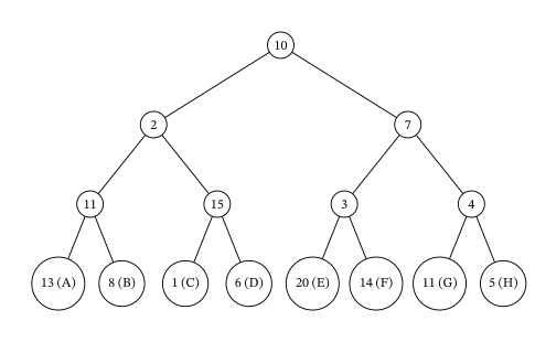
To be certain that you pick the branch with greatest sum, you could list each sum from each of the different branches:

A: $10 + 2 + 11 + 13 = 36$

B: $10 + 2 + 11 + 8 = 31$

C: $10 + 2 + 15 + 1 = 28$

D: $10 + 2 + 15 + 6 = 33$

E: $10 + 7 + 3 + 20 = 40$

F: $10 + 7 + 3 + 14 = 34$

G: $10 + 7 + 4 + 11 = 32$

H: $10 + 7 + 4 + 5 = 26$

Then we know with certainty that branch E has the greatest sum.

Figure 12.188 Branch E

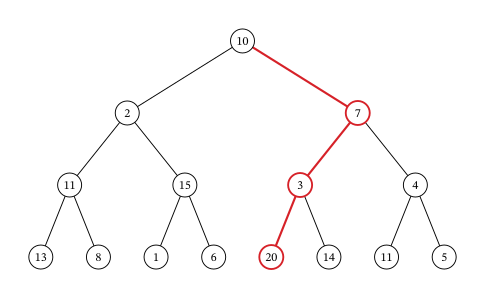
Now suppose that you wanted to find the branch with the highest value, but you only were shown the tree diagram in phases, one step at a time.

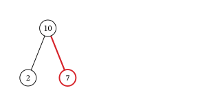
A graph has 3 vertices. The vertices are labeled 10, 2, and 7. 10 branches into 2 and 7. The edge, 10 to 7 is highlighted. — **Figure 12.189** Tree Diagram Phase 1

After phase 1, you would have chosen the branch with 10 and 7. So far, you are following the same branch. Let’s look at the next phase.

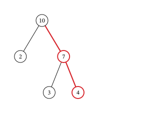
A graph has 5 vertices. The vertices are labeled 10, 2, 7, 3, and 4. 10 branches into 2 and 7. 7 branches into 3 and 4. The edges, 10 to 7 and 7 to 4 are highlighted. — **Figure 12.190** Tree Diagram Phase 2

After phase 2, based on the information you have, you will choose the branch with 10, 7 and 4. Now, you are following a different branch than before, but it is the best choice based on the information you have. Let’s look at the last phase.

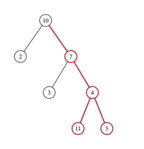
A graph has 7 vertices. The vertices are labeled 10, 2, 7, 3, 4, 11, and 15. 10 branches into 2 and 7. 7 branches into 3 and 4. 4 branches into 11 and 5. The edges, 10 to 7, 7 to 4, and 4 to 11 are highlighted. 11 and 5 are labeled G and H. — **Figure 12.191** Tree Diagram Phase 3

After phase 3, you will choose branch G which has a sum of 32.

The process of adding the values on each branch and selecting the highest sum is an example of a brute force algorithm because all options were explored in detail. The process of choosing the branch in phases, based on the best choice at each phase is a greedy algorithm. Although a brute force algorithm gives us the ideal solution, it can take a very long time to implement. Imagine a tree diagram with thousands or even millions of branches. It might not be possible to check all the sums. A greedy algorithm, on the other hand, can be completed in a relatively short time, and generally leads to good solutions, but not necessarily the ideal solution.

Example 1 Distinguishing between Brute Force and Greedy Algorithms

A cashier rings up a sale for $4.63 cents in U.S. currency. The customer pays with a $5 bill. The cashier would like to give the customer $0.37 in change using the fewest coins possible. The coins that can be used are quarters ($0.25), dimes ($0.10), nickels ($0.05), and pennies ($0.01). The cashier starts by selecting the coin of highest value less than or equal to $0.37, which is a quarter. This leaves $$ 0.37 - $ 0.25 = $ 0.12$ . The cashier selects the coin of highest value less than or equal to $0.12, which is a dime. This leaves $$ 0.12 - $ 0.10 = $ 0.02$ . The cashier selects the coin of highest value less than or equal to $0.02, which is a penny. This leaves $$ 0.02 - $ 0.01 = $ 0.01$ . The cashier selects the coin of highest value less than or equal to $0.01, which is a penny. This leaves no remainder. The cashier used one quarter, one dime, and two pennies, which is four coins. Use this information to answer the following questions.

Is the cashier’s approach an example of a greedy algorithm or a brute force algorithm? Explain how you know.
The cashier’s solution is the best solution. In other words, four is the fewest number of coins possible. Is this consistent with the results of an algorithm of this kind? Explain your reasoning.

The approach the cashier used is an example of a greedy algorithm, because the problem was approached in phases and the best choice was made at each phase. Also, it is not a brute force algorithm, because the cashier did not attempt to list out all possible combinations of coins to reach this conclusion.
Yes, it is consistent. A greedy algorithm does not always yield the best result, but sometimes it does.

The Traveling Salesperson Problem

Now let’s focus our attention on the graph theory application known as the traveling salesperson problem (TSP) in which we must find the shortest route to visit a number of locations and return to the starting point.

Recall from Hamilton Cycles, the officer in the U.S. Air Force who is stationed at Vandenberg Air Force base and must drive to visit three other California Air Force bases before returning to Vandenberg. The officer needed to visit each base once. We looked at the weighted graph in Figure 12.192 representing the four U.S. Air Force bases: Vandenberg, Edwards, Los Angeles, and Beal and the distances between them.

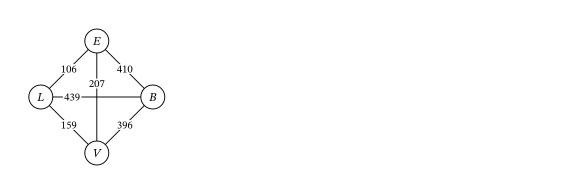
A graph represents the four California air force bases. The graph has four vertices: E, B, V, and L. The edge, E B is labeld 410 miles. The edge, B V is labeled 396 miles. The edge, V L is labeled 159 miles. The edge, L E is labeled 106 miles. The edge, L B is labeled 439 miles. The edge, E V is labeled 207 miles. — **Figure 12.192** Graph of Four California Air Force Bases

Any route that visits each base and returns to the start would be a Hamilton cycle on the graph. If the officer wants to travel the shortest distance, this will correspond to a Hamilton cycle of lowest weight. We saw in Table 12.11 that there are six distinct Hamilton cycles (directed cycles) in a complete graph with four vertices, but some lie on the same cycle (undirected cycle) in the graph.

**Table 12.11** Hamilton Cycles in a Complete Graph with Four Vertices
Complete Graph	Cycle	Cycle	Cycle

Clockwise Hamilton Cycle	a → b → c → d → a	a → b → d → c → a	a → c → b → d → a
Counterclockwise Hamilton Cycle	a → d → c → b → a	a → c → d → b → a	a → d → b → c → a

Since the distance between bases is the same in either direction, it does not matter if the officer travels clockwise or counterclockwise. So, there are really only three possible distances as shown in Figure 12.193.

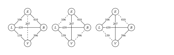
Three graphs represent the four California air force bases. Each graph has four vertices: E, B, V, and L. The edge, E B is labeled 410 miles. The edge, B V is labeled 396 miles. The edge, V L is labeled 159 miles. The edge, L E is labeled 106 miles. The edge, L B is labeled 439 miles. The edge, E V is labeled 207 miles. In the first graph, the edges, E V, and L B are in dashed lines. In the second graph, the edges, E L and B V are in dashed lines. In the third graph, the edges, E B and L V are in dashed lines. — **Figure 12.193** Three Possible Distances

The possible distances are:

$\begin{array}{l} 396 + 410 + 106 + 159 = 1071 \\ 207 + 410 + 439 + 159 = 1215 \\ 396 + 439 + 106 + 207 = 1148 \end{array}$

So, a Hamilton cycle of least weight is V → B → E → L → V (or the reverse direction). The officer should travel from Vandenberg to Beal to Edwards, to Los Angeles, and back to Vandenberg.

Finding Weights of All Hamilton Cycles in Complete Graphs

Notice that we listed all of the Hamilton cycles and found their weights when we solved the TSP about the officer from Vandenberg. This is a skill you will need to practice. To make sure you don't miss any, you can calculate the number of possible Hamilton cycles in a complete graph. It is also helpful to know that half of the directed cycles in a complete graph are the same cycle in reverse direction, so, you only have to calculate half the number of possible weights, and the rest are duplicates.

Example 2 Calculating Possible Weights of Hamilton Cycles

Suppose you have a complete weighted graph with vertices N, M, O, and P.

Use the formula $open parenthesis n minus 1 close parenthesis !$ to calculate the number of distinct Hamilton cycles in the graph.
Use the formula $\frac{(n - 1)!}{2}$ to calculate the greatest number of different weights possible for the Hamilton cycles.
Are all of the distinct Hamilton cycles listed here? How do you know?
Cycle 1: N → M → O → P → N
Cycle 2: N → M → P → O → N
Cycle 3: N → O → M → P → N
Cycle 4: N → O → P → M → N
Cycle 5: N → P → M → O → N
Cycle 6: N → P → O → M → N
Which pairs of cycles must have the same weights? How do you know?

There are 4 vertices; so, $n equals 4$ . This means there are $(n - 1)! = (4 - 1)! = 3 \cdot 2 \cdot 1 = 6$ distinct Hamilton cycles beginning at any given vertex.
Since $n equals 4$ , there are $\frac{(n - 1)!}{2} = \frac{(4 - 1)!}{2} = \frac{6}{2} = 3$ possible weights.
Yes, they are all distinct cycles and there are 6 of them.
Cycles 1 and 6 have the same weight, Cycles 2 and 4 have the same weight, and Cycles 3 and 5 have the same weight, because these pairs follow the same route through the graph but in reverse.

The Brute Force Method

The method we have been using to find a Hamilton cycle of least weight in a complete graph is a brute force algorithm, so it is called the brute force method. The steps in the brute force method are:

Step 1: Calculate the number of distinct Hamilton cycles and the number of possible weights.

Step 2: List all possible Hamilton cycles.

Step 3: Find the weight of each cycle.

Step 4: Identify the Hamilton cycle of lowest weight.

Example 3 Applying the Brute Force Method

On the next assignment, the air force officer must leave from Travis Air Force base, visit Beal, Edwards, and Vandenberg Air Force bases each exactly once and return to Travis Air Force base. There is no need to visit Los Angeles Air Force base. Use Figure 12.194 to find the shortest route.

Figure 12.194 Distances between Five California Air Force Bases

Step 1: Since there are 4 vertices, there will be $(4 - 1)! = 3! = 6$ cycles, but half of them will be the reverse of the others; so, there will be $\frac{(4 - 1)!}{2} = \frac{6}{2} = 3$ possible distances.

Step 2: List all the Hamilton cycles in the subgraph of the graph in Figure 12.195.

Figure 12.195 Subgraph with Cities B, E, T, and V

To find the 6 cycles, focus on the three vertices in the middle, B, E, and V. The arrangements of these vertices are BEV, BVE, EBV, EVB, VBE, and VEB. These would correspond to the 6 cycles:

1: T → B → E → V → T

2: T → B → V → E → T

3: T → E → B → V → T

4: T → E → V → B → T

5: T → V → B → E → T

6: T → V → E → B → T

Step 3: Find the weight of each path. You can reduce your work by observing the cycles that are reverses of each other.

1: $84 + 410 + 207 + 396 = 1097$

2: $84 + 396 + 207 + 370 = 1071$

3: $370 + 410 + 396 + 396 = 1572$

4: Reverse of cycle 2, 1071

5: Reverse of cycle 3, 1572

6: Reverse of cycle 1, 1097

Step 4: Identify a Hamilton cycle of least weight.

The second path, T → B → V → E → T, and its reverse, T → E → V → B → T, have the least weight. The solution is that the officer should travel from Travis Air Force base to Beal Air Force Base, to Vandenberg Air Force base, to Edwards Air Force base, and return to Travis Air Force base, or the same route in reverse.

Now suppose that the officer needed a cycle that visited all 5 of the Air Force bases in Figure 12.194. There would be $(5 - 1)! = 4! = 4 \times 3 \times 2 \times 1 = 24$ different arrangements of vertices and $\frac{(5 - 1)!}{2} = \frac{4!}{2} = \frac{24}{2} = 12$ distances to compare using the brute force method. If you consider 10 Air Force bases, there would be $(10 - 1)! = 9! = 9 \cdot 8 \cdot 7 \cdot 6 \cdot 5 \cdot 4 \cdot 3 \cdot 2 \cdot 1 = 362,880$ different arrangements and $\frac{(10 - 1)!}{2} = \frac{9!}{2} = \frac{9 \cdot 8 \cdot 7 \cdot 6 \cdot 5 \cdot 4 \cdot 3 \cdot 2 \cdot 1}{2} = 181,440$ distances to consider. There must be another way!

The Nearest Neighbor Method

When the brute force method is impractical for solving a traveling salesperson problem, an alternative is a greedy algorithm known as the nearest neighbor method, which always visit the closest or least costly place first. This method finds a Hamilton cycle of relatively low weight in a complete graph in which, at each phase, the next vertex is chosen by comparing the edges between the current vertex and the remaining vertices to find the lowest weight. Since the nearest neighbor method is a greedy algorithm, it usually doesn’t give the best solution, but it usually gives a solution that is "good enough." Most importantly, the number of steps will be the number of vertices. That’s right! A problem with 10 vertices requires 10 steps, not 362,880. Let’s look at an example to see how it works.

Suppose that a candidate for governor wants to hold rallies around the state. They plan to leave their home in city A, visit cities B, C, D, E, and F each once, and return home. The airfare between cities is indicated in the graph in Figure 12.196.

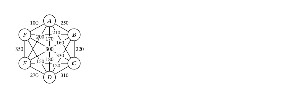
A graph represents the airfares between six different cities. The graph has 6 vertices. The vertices are A, B, C, D, E, and F. Edges from A leading to B, C, D, E, and F are labeled 250 dollars, 210 dollars, 300 dollars, 200 dollars, and 100 dollars. Edges from B leading to C, D, E, and F are labeled 220 dollars, 120 dollars, 160 dollars, and 170 dollars. Edges from C to D, E, and F are labeled 310 dollars, 180 dollars, and 330 dollars. Edges from D to E and F 270 dollars and 150 dollars. An edge from E to F is labeled 350 dollars. — **Figure 12.196** Airfares between Cities *A, B, C, D, E*, and F

Let’s help the candidate keep costs of travel down by applying the nearest neighbor method to find a Hamilton cycle that has a reasonably low weight. Begin by marking starting vertex as $V sub 1$ for "visited 1st." Then to compare the weights of the edges between A and vertices adjacent to A: $250, $210, $300, $200, and $100 as shown in Figure 12.197. The lowest of these is $100, which is the edge between A and F.

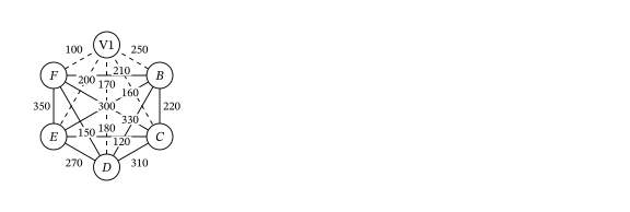
Mark F as $V sub 2$ for "visited 2nd" then compare the weights of the edges between F and the remaining vertices adjacent to F: $170, $330, $150 and $350 as shown in Figure 12.198. The lowest of these is $150, which is the edge between F and D.

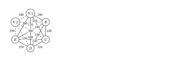
Mark D as $V sub 3$ for "visited 3rd." Next, compare the weights of the edges between D and the remaining vertices adjacent to D: $120, $310, and $270 as shown in Figure 12.199. The lowest of these is $120, which is the edge between D and B.

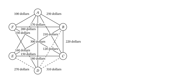
So, mark B as $V sub 4$ for "visited 4th." Finally, compare the weights of the edges between B and the remaining vertices adjacent to B: $160 and $220 as shown in Figure 12.200. The lower amount is $160, which is the edge between B and E.

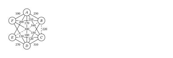
Now you can mark E as $V sub 5$ and mark the only remaining vertex, which is C, as $V sub 6$ . This is shown in Figure 12.201. Make a note of the weight of the edge from E to C, which is $180, and from C back to A, which is $210.

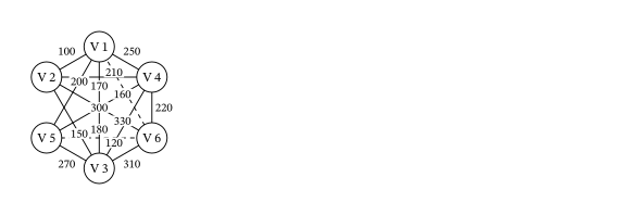
The Hamilton cycle we found is A → F → D → B → E → C → A. The weight of the circuit is $$ 100 + $ 150 + $ 120 + $ 160 + $ 180 + $ 210 = $ 920$ . This may or may not be the route with the lowest cost, but there is a good chance it is very close since the weights are most of the lowest weights on the graph and we found it in six steps instead of finding 120 different Hamilton cycles and calculating 60 weights. Let’s summarize the procedure that we used.

Step 1: Select the starting vertex and label $V sub 1$ for "visited 1st." Identify the edge of lowest weight between $V sub 1$ and the remaining vertices.

Step 2: Label the vertex at the end of the edge of lowest weight that you found in previous step as $V_{n}$ where the subscript n indicates the order the vertex is visited. Identify the edge of lowest weight between $V_{n}$ and the vertices that remain to be visited.

Step 3: If vertices remain that have not been visited, repeat Step 2. Otherwise, a Hamilton cycle of low weight is $V sub 1 → V sub 2 → ⋯ → V sub n → V sub 1$ .

Example 4 Using the Nearest Neighbor Method

Suppose that the candidate for governor wants to hold rallies around the state but time before the election is very limited. They would like to leave their home in city A, visit cities B, C, D, E, and F each once, and return home. The airfare between cities is not as important as the time of travel, which is indicated in Figure 12.202. Use the nearest neighbor method to find a route with relatively low travel time. What is the total travel time of the route that you found?

Figure 12.202 Travel Times between Cities A, B, C, D, E and F

Step 1: Label vertex A as $V sub 1$ . The edge of lowest weight between A and the remaining vertices is 85 min between A and D.

Step 2: Label vertex D as $V sub 2$ . The edge of lowest weight between D and the vertices that remain to be visited, B, C, E, and F, is 70 min between D and F.

Repeat Step 2: Label vertex F as $V sub 3$ . The edge of lowest weight between F and the vertices that remain to be visited, B, C, and E, is 75 min between F and C.

Repeat Step 2: Label vertex C as $V sub 4$ . The edge of lowest weight between C and the vertices that remain to be visited, B and E, is 100 min between C and B.

Repeat Step 2: Label vertex B as $V sub 5$ . The only vertex that remains to be visited is E. The weight of the edge between B and E is 95 min.

Step 3: A Hamilton cycle of low weight is A → D → F → C → B → E → A. So, a route of relatively low travel time is A to D to F to C to B to E and back to A. The total travel time of this route is: $85 \min + 70 \min + 75 \min + 100 \min + 95 \min + 90 \min = 515 \min or 8 hrs 35 \min$

Key Terms

brute force algorithm
greedy algorithm
traveling salesperson problem (TSP)
brute force method
nearest neighbor method

Key Concepts

A brute force algorithm always finds the ideal solution but can be impractical whereas a greedy algorithm is efficient but usually does not lead to the ideal solution.
A Hamilton cycle of lowest weight is a solution to the traveling salesperson problem.
The brute force method finds a Hamilton cycle of lowest weight in a complete graph.
The nearest neighbor method is a greedy algorithm that finds a Hamilton cycle of relatively low weight in a complete graph.

Formulas

In a complete graph with $n$ vertices, the number of distinct Hamilton cycles is $open parenthesis n minus 1 close parenthesis !$ .
In a complete graph with $n$ vertices, there are at most $\frac{(n - 1)!}{2}$ different weights of Hamilton cycles.

Adapted from Contemporary Mathematics by OpenStax (openstax.org), licensed under CC BY-NC-SA 4.0. Changes were made. License: CC-BY-NC-SA-4.0.