8.6 The Normal Distribution

Learning Objectives

After completing this section, you should be able to:

1. Describe the characteristics of the normal distribution.
2. Apply the 68-95-99.7 percent groups to normal distribution datasets.
3. Use the normal distribution to calculate a $z$-score.
4. Find and interpret percentiles and quartiles.

Moving Toward Normality

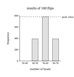
Let’s take a look at a histogram for the dataset in our section opener:

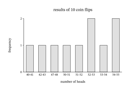
This is interesting, but the data seem pretty sparse. There were no trials where you saw between 43 and 47 heads, for example. Those results don’t seem impossible; we just didn’t flip enough times to give them a chance to pop up. So, let’s do it again, but this time we'll perform 100 coin flips 100 times. Rather than review all 100 results, which could be overwhelming, let's instead visualize the resulting histogram.

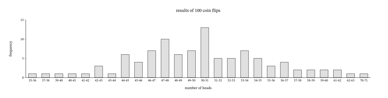
From the histogram, we see that most of the trials resulted in between, say, 44 and 56 heads. There were some more unusual results: one trial resulted in 70 heads, which seems really unlikely (though still possible!). But we’re starting to maybe get a sense of the distribution. More data would help, though. Let’s simulate another 900 trials and add them to the histogram!

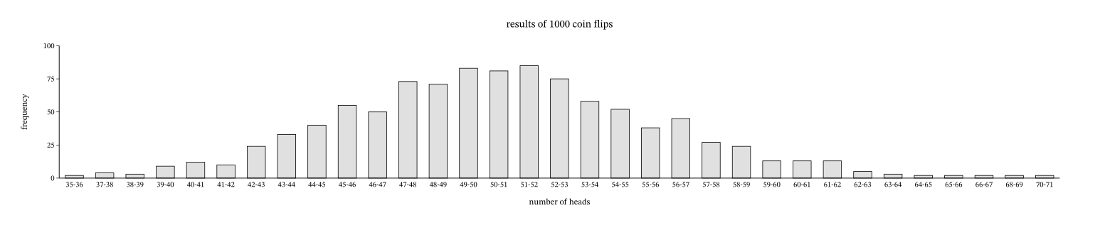
We can still see that 70 is a really unusual observation, though we came close in another trial (one that had 68 heads). Now, the distribution is coming more into focus: It looks quite symmetric and bell-shaped. Let’s just go ahead and take this thought experiment to an extreme conclusion: 10,000 trials.

The distribution is pretty clear now. Distributions that are symmetric and bell-shaped like this pop up in all sorts of natural phenomena, such as the heights of people in a population, the circumferences of eggs of a particular bird species, and the numbers of leaves on mature trees of a particular species. All of these have bell-shaped distributions. Additionally, the results of many types of repeated experiments generally follow this same pattern, as we saw with the coin-flipping example; this fact is the basis for much of the work done by statisticians. It’s a fact that’s important enough to have its own name: the Central Limit Theorem.

The Normal Distribution

In the coin flipping example above, the distribution of the number of heads for 10,000 trials was close to perfectly symmetric and bell-shaped:

Because distributions with this shape appear so often, we have a special name for them: normal distributions. Normal distributions can be completely described using two numbers we’ve seen before: the mean of the data and the standard deviation of the data. You may remember that we described the mean as a measure of centrality; for a normal distribution, the mean tells us exactly where the center of the distribution falls. The peak of the distribution happens at the mean (and, because the distribution is symmetric, it’s also the median). The standard deviation is a measure of dispersion; for a normal distribution, it tells us how spread out the histogram looks. To illustrate these points, let’s look at some examples.

Let’s put it all together to identify a completely unknown normal distribution.

Properties of Normal Distributions: The 68-95-99.7 Rule

The most important property of normal distributions is tied to its standard deviation. If a dataset is perfectly normally distributed, then 68% of the data values will fall within one standard deviation of the mean. For example, suppose we have a set of data that follows the normal distribution with mean 400 and standard deviation 100. This means 68% of the data would fall between the values of 300 (one standard deviation below the mean: $400-100=300$) and 500 (one standard deviation above the mean: $400+100=500$). Looking at the histogram below, the shaded area represents 68% of the total area under the graph and above the axis:

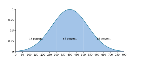
Since 68% of the area is in the shaded region, this means that $100\%-68\%=32\%$ of the area is found in the unshaded regions. We know that the distribution is symmetric, so that 32% must be divided evenly into the two unshaded tails: 16% in each.

Of course, datasets in the real world are never perfect; when dealing with actual data that seem to follow a symmetric, bell-shaped distribution, we’ll give ourselves a little bit of wiggle room and say that approximately 68% of the data fall within one standard deviation of the mean.

The rule for one standard deviation can be extended to two standard deviations. Approximately 95% of a normally distributed dataset will fall within 2 standard deviations of the mean. If the mean is 400 and the standard deviation is 100, that means 95% calculation describes the way we compute standardized scores. (two standard deviations below the mean: $400-2\times 100=200$) and 600 (two standard deviations above the mean: $400+2\times 100=600$). We can visualize this in the following histogram:

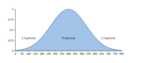
As before, since 95% of the data are in the shaded area, that leaves 5% of the data to go into the unshaded tails. Since the histogram is symmetric, half of the 5% (that’s 2.5%) is in each.

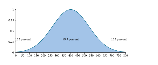
We can even take this one step further: 99.7% of normally distributed data fall within 3 standard deviations of the mean. In this example, we’d see 99.7% of the data between 100 (calculated as $400-3\times 100=100$) and 700 (calculated as $400+3\times 100=700$). We can see this in the histogram below, although you may need to squint to find the unshaded bits in the tails!

This observation is formally known as the 68-95-99.7 Rule.

There are more problems we can solve using the 68-95-99.7 Rule. but first we must understand what the rule implies. Remember, the rule says that 68% of the data falls within one standard deviation of the mean. Thus, with normally distributed data with mean 100 and standard deviation 10, we have this distribution:

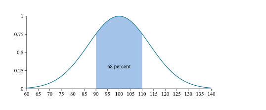
Since we know that 68% of the data lie within one standard deviation of the mean, the implication is that 32% of the data must fall beyond one standard deviation away from the mean. Since the histogram is symmetric, we can conclude that half of the 32% (or 16%) is more than one standard deviation above the mean and the other half is more than one standard deviation below the mean:

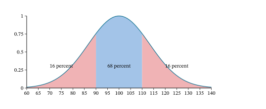
Further, we know that the middle 68% can be split in half at the peak of the histogram, leaving 34% on either side:

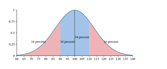
So, just the “68” part of the 68-95-99.7 Rule gives us four other proportions in addition to the 68% in the rule. Similarly, the “95” and “99.7” parts each give us four more proportions:

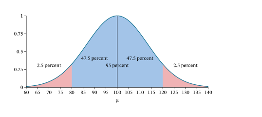
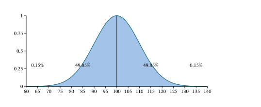
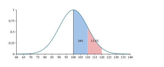
We can put all these together to find even more complicated proportions. For example, since the proportion between 100 and 120 is 47.5% and the proportion between 100 and 110 is 34%, we can subtract to find that the proportion between 110 and 120 is $47.5-34=13.5\%$:

Standardized Scores

When we want to apply the 68-95-99.7 Rule, we must first figure out how many standard deviations above or below the mean our data fall. This calculation is common enough that it has its own name: the standardized score. Values above the mean have positive standardized scores, while those below the mean have negative standardized scores. Since it's common to use the letter $z$ to represent a standard score, this value is also often referred to as a $\mathit{z}$-score.

So far, we’ve only really considered $z$-scores that are whole numbers, but in general they can be any number at all. For example, if we have data that are normally distributed with mean 80 and standard deviation 6, the value 85 is five units above the mean, which is less than one standard deviation. Dividing by the standard deviation, we get $\frac{5}{6}$. Since 85 is $\frac{5}{6}$ of one standard deviation above the mean, we’d say that the standardized score for 85 is $z=\frac{5}{6}$ (which is positive, since $85>80$). This calculation describes the way we compute standardized scores.

Using Google Sheets to Find Normal Percentiles

The 68-95-99.7 Rule is great when we’re dealing with whole-number $z$-scores. However, if the $z$-score is not a whole number, the Rule isn’t going to help us. Luckily, we can use technology to help us out. We’ll talk here about the built-in functions in Google Sheets, but other tools work similarly.

Let’s say we’re working with normally distributed data with mean 40 and standard deviation 7, and we want to know at what percentile a data value of 50 would fall. That corresponds to finding the proportion of the data that are less than 50. If we create our histogram and mark off whole-number multiples of the standard deviation like we did before, we’ll see why the 68-95-99.7 Rule isn’t going to help:

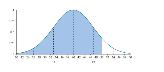
Since 50 doesn’t line up with one of our lines, the 68-95-99.7 Rule fails us. Looking back at Figure 8.48 and Figure 8.49, the best we can say is that 50 is between the 84th and 99.5th percentiles, but that’s a pretty wide range. Google Sheets has a function that can help; it’s called NORM.DIST. Here’s how to use it:

1. Click in an empty cell in your worksheet.
2. Type “=NORM.DIST(“
3. Inside the parentheses, we must enter a list of four things, separated by commas: the data value, the mean, the standard deviation, and the word “TRUE”. These have to be entered in this order!
4. Close the parentheses, and hit Enter. The result is then displayed in the cell; convert it to a percent to get the percentile.

So, for our example, we should type “=NORM.DIST(50, 40, 7, TRUE)” into an empty cell, and hit Enter. The result is 0.9234362745; converting to a percent and rounding, we can conclude that 50 is at the 92nd percentile. Let’s walk through a few more examples.

Google Sheets can also help us go the other direction: If we want to find the data value that corresponds to a given percentile, we can use the NORM.INV function. For example, if we have normally distributed data with mean 150 and standard deviation 25, we can find the data value at the 30th percentile as follows:

1. Click on an empty cell in your worksheet.
2. Type “=NORM.INV(“
3. Inside the parentheses, we’ll enter a list of three numbers, separated by commas: the percentile in question expressed as a decimal, the mean, and the standard deviation. These must be entered in this order!
4. Close the parentheses and hit Enter. The desired data value will be in the cell!

In our example, we want the 30th percentile; converting 30% to a decimal gives us 0.3. So, we’ll type “=NORM.INV(0.3, 150, 25)” to get 136.8899872; let’s round that off to 137.

Key Concepts

• Normally distributed data follow a bell-shaped, symmetrical distribution.
• The mean of normally distributed data falls at the peak of the distribution. The standard deviation of normally-distributed data is the distance from the peak to either of the inflection points.
• Data that are normally distributed follow the 68-95-99.7 Rule, which says that approximately 68% of the data fall within one standard deviation of the mean, 95% fall within two standard deviations, and 99.7% fall within three standard deviations.
• The $z$-score for a data value is the number of standard deviations that value falls above (or below, if the $z$-score is negative) the mean.
• We can use the normal distribution to estimate percentiles.

Formulas

If $x$ is a member of a normally distributed dataset with mean $\mu$ and standard deviation $\sigma$, then the standardized score for $x$ is

$$z=\frac{x-\mu }{\sigma }.$$

If you know a $z$-score but not the original data value $x$, you can find it by solving the previous equation for $x$:

$$x=\mu +z\times \sigma .$$