
5.5 Graphing Linear Equations and Inequalities

Learning Objectives
After completing this section, you should be able to:
- Graph linear equations and inequalities in two variables.
- Solve applications of linear equations and inequalities.
In this section, we will learn how to graph linear equations and inequalities. There are several real-world scenarios that can be represented by graphs of linear inequalities. Think of filling your car up with gasoline. If gasoline is $3.99 per gallon and you put 10 gallons in your car, you will pay $39.90. Your friend buys 15 gallons of gasoline and pays $59.85. You can plot these points on a coordinate system and connect the points with a line to create the graph of a line. You'll learn to do both in this section.
Plotting Points on a Rectangular Coordinate System
Just like maps use a grid system to identify locations, a grid system is used in algebra to show a relationship between two variables in a rectangular coordinate system. The rectangular coordinate system is also called the -plane or the “coordinate plane.”
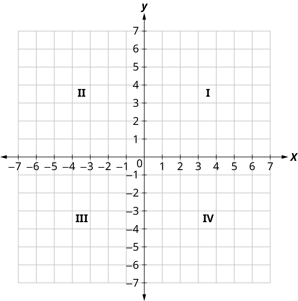
The rectangular coordinate system is formed by two intersecting number lines, one horizontal and one vertical. The horizontal number line is called the -axis. The vertical number line is called the -axis. These axes divide a plane into four regions, called quadrants. The quadrants are identified by Roman numerals, beginning on the upper right and proceeding counterclockwise. See Figure 5.19.
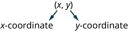
In the rectangular coordinate system, every point is represented by an ordered pair (Figure 5.20). The first number in the ordered pair is the -coordinate of the point, and the second number is the -coordinate of the point. The phrase "ordered pair" means that the order is important. At the point where the axes cross and where both coordinates are zero, the ordered pair is . The point has a special name. It is called the origin.
We use the coordinates to locate a point on the -plane. Let's plot the point as an example. First, locate 1 on the -axis and lightly sketch a vertical line through . Then, locate 3 on the -axis and sketch a horizontal line through . Now, find the point where these two lines meet—that is the point with coordinates . See Figure 5.21.
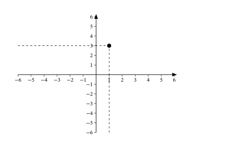
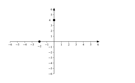
Notice that the vertical line through and the horizontal line through are not part of the graph. The dotted lines are just used to help us locate the point . When one of the coordinates is zero, the point lies on one of the axes. In Figure 5.22, the point is on the -axis and the point (−2, 0) is on the -axis.
Graphing Linear Equations in Two Variables
Up to now, all the equations you have solved were equations with just one variable. In almost every case, when you solved the equation, you got exactly one solution. But equations can have more than one variable. Equations with two variables may be of the form . An equation of this form, where and are both not zero, is called a linear equation in two variables. Here is an example of a linear equation in two variables, and .
The equation is also a linear equation. But it does not appear to be in the form . We can use the addition property of equality and rewrite it in form.
Step 1: Add to both sides.
Step 2: Simplify.
Step 3: Put it in form.
By rewriting as , we can easily see that it is a linear equation in two variables because it is of the form . When an equation is in the form , we say it is in standard form of a linear equation. Most people prefer to have , , and be integers and when writing a linear equation in standard form, although it is not strictly necessary.
Linear equations have infinitely many solutions. For every number that is substituted for there is a corresponding value. This pair of values is a solution to the linear equation and is represented by the ordered pair (,). When we substitute these values of and into the equation, the result is a true statement, because the value on the left side is equal to the value on the right side.
We can plot these solutions in the rectangular coordinate system. The points will line up perfectly in a straight line. We connect the points with a straight line to get the graph of the linear equation. We put arrows on the ends of each side of the line to indicate that the line continues in both directions.
A graph is a visual representation of all the solutions of a linear equation. The line shows you all the solutions to that linear equation. Every point on the line is a solution of that linear equation. And every solution of the linear equation is on this line. This line is called the graph of the equation. Points not on the line are not solutions! The graph of a linear equation is a straight line.
- Every point on the line is a solution of the equation.
- Every solution of this equation is a point on this line.
The steps to take when graphing a linear equation by plotting points are:
Step 1: Find three points whose coordinates are solutions to the equation. Organize them in a table.
Step 2: Plot the points in a rectangular coordinate system. Check that the points line up. If they do not, carefully check your work.
Step 3: Draw the line through the three points. Extend the line to fill the grid and put arrows on both ends of the line.
It is true that it only takes two points to determine a line, but it is a good habit to use three points. If you only plot two points and one of them is incorrect, you can still draw a line, but it will not represent the solutions to the equation. It will be the wrong line. If you use three points, and one is incorrect, the points will not line up. This tells you something is wrong, and you need to check your work.
Solving Applications Using Linear Equations in Two Variables
Many fields use linear equalities to model a problem. While our examples may be about simple situations, they give us an opportunity to build our skills and to get a feel for how they might be used.
Graphing Linear Inequalities
Previously we learned to solve inequalities with only one variable. We will now learn about inequalities containing two variables that can be written in one of the following forms: , , , and where and are not both zero. We will look at linear inequalities in two variables, which are very similar to linear equations in two variables.
Like linear equations, linear inequalities in two variables have many solutions. Any ordered pair (, ) that makes an inequality true when we substitute in the values is a solution to a linear inequality.
Let us think about . The point separated that number line into two parts. On one side of 3 are all the numbers less than 3. On the other side of 3 all the numbers are greater than 3. See Figure 5.29.
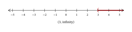
Similarly, the line separates the plane into two regions. On one side of the line are points with . On the other side of the line are the points with . We call the line a boundary line.
For an inequality in one variable, the endpoint is shown with a parenthesis (Figure 5.30) or a bracket (Figure 5.31) depending on whether or not is included in the solution:


Similarly, for an inequality in two variables, the boundary line is shown with a solid or dashed line to show whether or not it the line is included in the solution.
| Boundary line is | Boundary line is |
| Boundary line is not included in solution. | Boundary line is included in solution. |
| Boundary line is dashed. | Boundary line is solid. |
Now, let us take a look at what we found in Example 5.43. We will start by graphing the line , and then we will plot the five points we tested, as graphed in Figure 5.32. We found that some of the points were solutions to the inequality and some were not. Which of the points we plotted are solutions to the inequality ? The points and are solutions to the inequality . Notice that they are both on the same side of the boundary line . The two points and are on the other side of the boundary line , and they are not solutions to the inequality . For those two points, . What about the point ? Because , the point is a solution to the equation , but not a solution to the inequality . So, the point is on the boundary line.
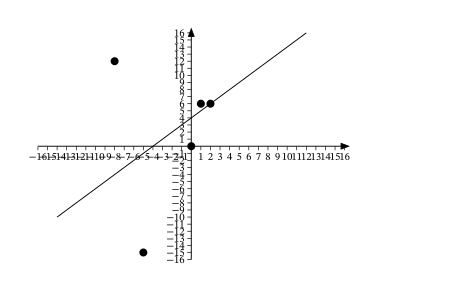
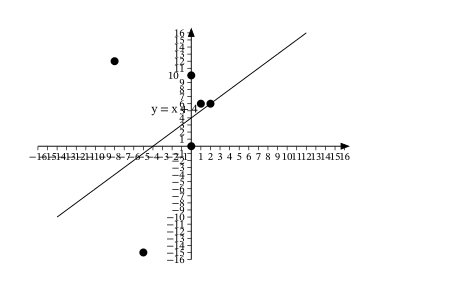
Let us take another point above the boundary line and test whether or not it is a solution to the inequality . The point clearly looks to be above the boundary line, doesn’t it? Is it a solution to the inequality?
Yes, is a solution to . Any point you choose above the boundary line is a solution to the inequality . All points above the boundary line are solutions. Similarly, all points below the boundary line, the side with and , are not solutions to , as shown in Figure 5.33.
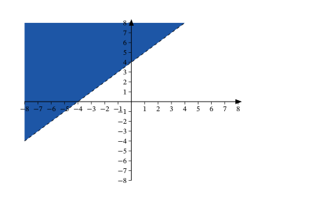
The graph of the inequality is shown in Figure 5.34. The line divides the plane into two regions. The shaded side shows the solutions to the inequality . The points on the boundary line, those where , are not solutions to the inequality , so the line itself is not part of the solution. We show that by making the boundary line dashed, not solid.
Solving Applications Using Linear Inequalities in Two Variables
Many fields use linear inequalities to model a problem. While our examples may be about simple situations, they give us an opportunity to build our skills and to get a feel for how they might be used.
Key Terms
- ordered pair
- origin
- points on the axes
- linear equation in two variables
- standards form of a linear equation
- solution
- linear inequality in two variables
- solution to a linear inequality
- boundary line
Key Concepts
- Linear equations can be represented graphically on a rectangular coordinate system.
- Solving linear equations in two variables means finding the point where two lines intersect. There are three possibilities: The lines intersect at exactly one point; the lines do not intersect (they are parallel); or the lines intersect everywhere (they are the same line).
- Solving linear inequalities in two variables means finding a region of possible answers. Every point in this region will make both inequalities true statements.
- Plotting points is a standard way to help graph linear equations and linear inequalities.
Videos
- Graphing Linear Inequalities in Two Variables ↗ new tab
Adapted from Contemporary Mathematics by OpenStax (openstax.org), licensed under CC BY-NC-SA 4.0. Changes were made. License: CC-BY-NC-SA-4.0.