
5.8 Graphing Functions
Learning Objectives
After completing this module, you should be able to:
- Graph functions using intercepts.
- Compute slope.
- Graph functions using slope and -intercept.
- Graph horizontal and vertical lines.
- Interpret graphs of functions.
- Model applications using slope and -intercept.
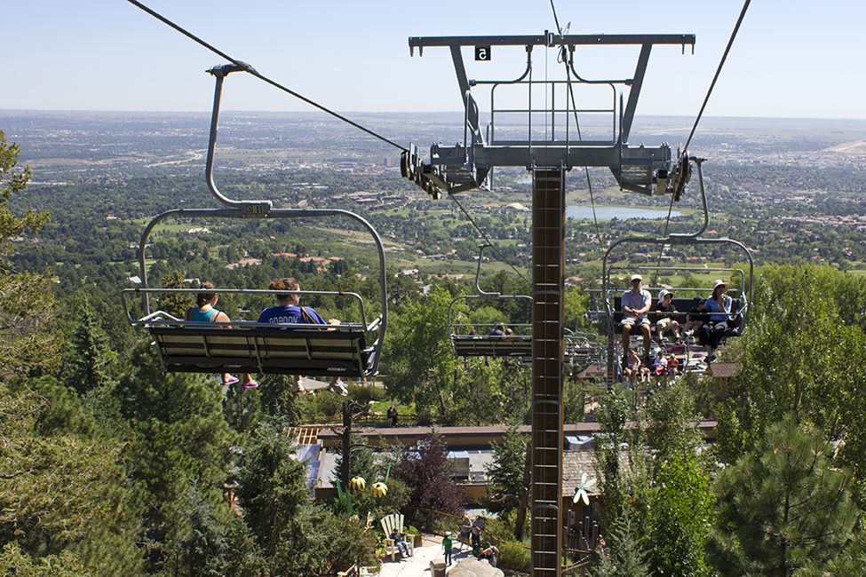
In this section, we will expand our knowledge of graphing by graphing linear functions. There are many real-world scenarios that can be represented by graphs of linear functions. Imagine a chairlift going up at a ski resort. The journey a skier takes travelling up the chairlift could be represented as a linear function with a positive slope. The journey a skier takes down the slopes could be represented by a linear function with a negative slope.
Graphing Functions Using Intercepts
Every linear equation can be represented by a unique line that shows all the solutions of the equation. We have seen that when graphing a line by plotting points, you can use any three solutions to graph. This means that two people graphing the line might use different sets of three points. At first glance, their two lines might not appear to be the same, since they would have different points labeled. But if all the work was done correctly, the lines should be exactly the same. One way to recognize that they are indeed the same line is to look at where the line crosses the -axis and the -axis. These points are called the intercepts of a line. Let us review the graphs of the lines in Figure 5.63.

The table below lists where each of these lines crosses the - and -axis. Do you see a pattern? For each line, the -coordinate of the point where the line crosses the -axis is zero. The point where the line crosses the -axis has the form and is called the -intercept of the line. The -intercept occurs when is zero. In each line, the -coordinate of the point where the line crosses the -axis is zero. The point where the line crosses the -axis has the form and is called the -intercept of the line. The -intercept occurs when is zero.
| Figure | The line crosses the at: | Ordered Pair for this Point | The line crosses the at: | Ordered Pair for This Point |
|---|---|---|---|---|
| Figure (a) | 3 | 6 | ||
| Figure (b) | 4 | |||
| Figure (c) | 5 | |||
| Figure (d) | 0 | 0 | ||
| General Figure |
Computing Slope
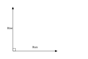
When graphing linear equations, you may notice that some lines tilt up as they go from left to right and some lines tilt down. Some lines are very steep and some lines are flatter. In mathematics, the measure of the steepness of a line is called the slope of the line. To find the slope of a line, we locate two points on the line whose coordinates are integers. Then we sketch a right triangle where the two points are vertices of the triangle and one side is horizontal and one side is vertical. Next, we measure or calculate the distance along the vertical and horizontal sides of the triangle. The vertical distance is called the rise and the horizontal distance is called the run.
We can assign a numerical value to the slope of a line by finding the ratio of the rise and run. The rise is the amount the vertical distance changes while the run measures the horizontal change, as shown in this illustration. Slope (Figure 5.66) is a rate of change.
The concept of slope has many applications in the real world. In construction, the pitch of a roof, the slant of plumbing pipes, and the steepness of stairs are all applications of slope. As you ski or jog down a hill, you definitely experience slope.
Sometimes we will need to find the slope of a line between two points when we don’t have a graph to measure the rise and the run. We could plot the points on grid paper, then count out the rise and the run, but there is a way to find the slope without graphing. First, we need to introduce some algebraic notation.
We have seen that an ordered pair (, ) gives the coordinates of a point. But when we work with slopes, we use two points. How can the same symbol (, ) be used to represent two different points? Mathematicians use subscripts to distinguish such points. For example, (, ) would be said aloud as “ sub 1, sub 1” and (, ) read “ sub 2, sub 2.” The “sub” is a short way of saying “subscript.” We will use (, ) to identify the first point and (, ) to identify the second point in our slope equation. If we had more than two points, (if we were finding more than one slope), we could use (, ), (, ), and so on.
Let’s review how the rise and run relate to the coordinates of the two points by taking another look at the slope of the line between the points and , as shown in Figure 5.69.
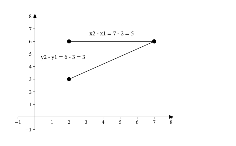
On the graph, we count the rise of 3 and the run of 5. Notice on the graph that that (, ) is the point and (, ) is the point . The rise can be found by subtracting the -coordinates, 6 and 3, and the run can be found by subtracting the -coordinates 7 and 2.
We have shown that is really another version of . We can use this formula to find the slope of a line.
Graphing Functions Using Slope and -Intercept
We have graphed linear equations by plotting points and using intercepts. Once we see how an equation in slope-intercept form and its graph are related, we will have one more method we can use to graph lines. Review the graph of the equation in Figure 5.71 and find its slope and -intercept.
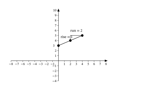
The vertical and horizontal lines in the graph show us the rise is 1 and the run is 2, respectively.
Substituting into the slope formula:
The -intercept is . Look at the equation of this line.
Look at the slope and -intercept.
When a linear equation is solved for , the coefficient of the term is the slope and the constant term is the -coordinate of the -intercept. We say that the equation is in slope-intercept form. Sometimes the slope-intercept form is called the -form.
Graphing Horizontal and Vertical Lines
Some linear equations have only one variable. They may have just without the , or just without an . This changes how we make a table of values to get the points to plot. Let us consider the equation . This equation has only one variable, . The equation says that is always equal to , so its value does not depend on . No matter what the value of is, the value of is always . To make a table of values, write in for all the -values. Then choose any values for . Since does not depend on , you can choose any numbers you like. But to fit the points on our coordinate graph, we will use 1, 2, and 3 for the -coordinates in the table below.
| (, ) | ||
| −3 | 1 | |
| 2 | ||
| 3 | ||
Plot the points from the table and connect them with a straight line (Figure 5.73). Notice that we have graphed a vertical line.
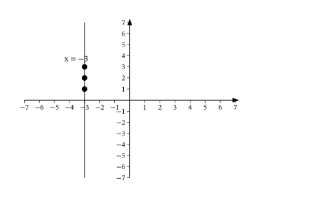
What is the slope? If we take the two points and then the rise is 2 and the run is 0.
Using the slope formula we get:
The slope is undefined since division by zero is undefined. We say that the slope of the vertical line is undefined. The slope of any vertical line (where is any number) will be undefined.
What if the equation has but no ? Let’s graph the equation . This time the -value is a constant, so in this equation, does not depend on . Fill in 4 for all the values in the table below and then choose any values for . We will use 0, 2, and 4 for the -coordinates.
| (, ) | ||
| 0 | 4 | |
| 2 | 4 | |
| 4 | 4 |
In Figure 5.74, we have graphed a horizontal line passing through the -axis at 4.
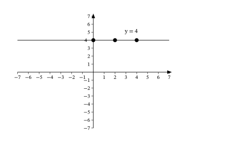
What is the slope? If we take the two points and then the rise is 0 and the run is 2. Using the slope formula, we get . The slope of the horizontal line is 0. The slope of any horizontal line (where is any number) will be 0. When the -coordinates are the same, the rise is 0.
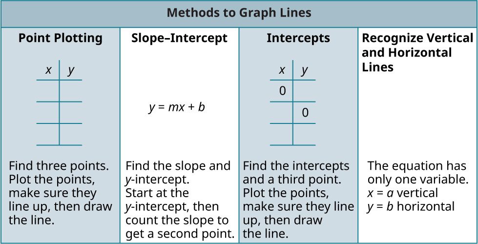
The table below summarizes all the methods we have used to graph lines.
Interpreting Graphs of Functions
An important yet often overlooked area in algebra involves interpreting graphs. Oftentimes in math classes, students are given mathematical functions and can make graphs to represent them. But the interpretation of graphs is a more applicable skill to the real world. Being able to “read” a graph—understanding its domain and range, what the intercepts mean, and what the slope (or curve) means— that's a real-world skill.
Modeling Applications Using Slope and -Intercept
Many real-world applications are modeled by linear equations. We will review a few applications here so you can understand how equations written in slope-intercept form relate to real-world situations. Usually when a linear equation model uses real-world data, different letters are used for the variables instead of using only and . The variable names often remind us of what quantities are being measured. Also, we often need to extend the axes in our rectangular coordinate system to bigger positive and negative numbers to accommodate the data in the application.
Key Terms
- intercepts of a line
- slope
- slope-intercept form
Key Concepts
- Every linear function can be graphically represented by a unique line that shows all the solutions of the equation.
- The points where the graph of a line intersects the -axis and -axis are called the intercepts of the line.
- Most lines will have one -intercept and one -intercept. Only if the line is straight vertical (no -intercept) or straight horizontal (no -intercept) will it not have both intercepts. Note that a line that is straight vertical is not a function, but a line that is straight horizontal is a function.
- Since any two points determine a straight line, any linear function can be graphed if both intercepts are known.
- The slope of a linear function is the ratio of the vertical change divided by the horizontal change. It is often referred to as .
- A formula for finding the slope of linear functions is for any two points of the linear function and .
Formulas
- To calculate slope , use the formula
,
where the rise measures the vertical change and the run measures the horizontal change. - To find the slope of the line between two points and , use the formula
Adapted from Contemporary Mathematics by OpenStax (openstax.org), licensed under CC BY-NC-SA 4.0. Changes were made. License: CC-BY-NC-SA-4.0.