12.3 Comparing Graphs

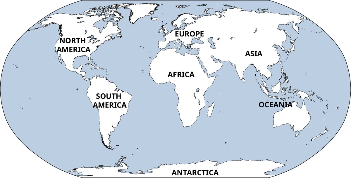
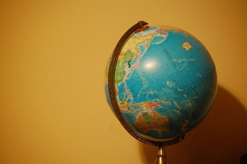
A map of the world continents. The continents are North America, South America, Europe, Asia, Africa, Oceania, and Antarctica. — **Figure 12.36** A flat map represents the surface of Earth in two dimensions.A flat map represents the surface of Earth in two dimensions. (credit: modification of work "World Map" by Scratchinghead/Wikimedia Commons, Public Domain)

A globe. — **Figure 12.37** A globe represents the surface of Earth in three dimensions.A globe represents the surface of Earth in three dimensions. (credit: "Globe" by Wendy Cope/Flickr, CC BY 2.0)

Learning Objectives

After completing this section, you should be able to:

Identify the characteristics used to compare graphs.
Determine when two graphs represent the same relationships
Explore real-world examples of graph isomorphisms
Find the complement of a graph

Maps of the same region may not always look the same. For example, a map of Earth on a flat surface looks distorted at the poles. When the same regions are mapped on a spherical globe, the countries that are closer to the polls appear smaller without the distortion. Despite these differences, the two maps still communicate the same relationships between nations such as shared boundaries, and relative position on the earth. In essence, they are the same map. This means that for every point on one map, there is a corresponding point on the other map in the same relative location. In this section, we will determine exactly what characteristics need to be the shared by two graphs in order for us to consider them “the same.”

When Are Two Graphs Really the Same Graph?

In arithmetic, when two numbers have the same value, we say they are equal, like ½ = 0.5. Although ½ and 0.5 look different, they have the same value, because they are assigned the same position on the real number line. When do we say that two graphs are equal?

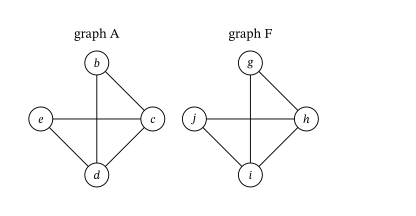
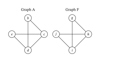
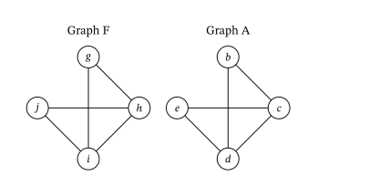
Figure 12.38 shows Graphs A and F, which are identical except for the labels. Graphs are visual representations of connections. As long as two graphs indicate the same pattern of connections, like Graph A and Graph F, they are considered to be equal, or in graph theory terms, isomorphic.

Two graphs are labeled graph A and graph F. Graph A has four vertices: b, c, d, and e. The edges connect b c, c e, e d, d b, and d c. Graph F has four vertices: g, h, i, and j. The edges connect g h, h j, j i, I g, and I h. — **Figure 12.38** Identical Graphs with Different Labels

Two graphs are isomorphic if either one of these conditions holds:

One graph can be transformed into the other without breaking existing connections or adding new ones.
There is a correspondence between their vertices in such a way that any adjacent pair in one graph corresponds to an adjacent pair in the other graph.

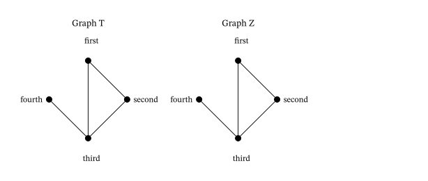
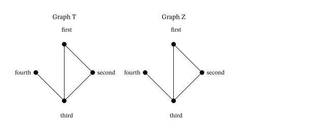
It is important to note that if either one of the isomorphic conditions holds, then both of them do. When we need to decide if two graphs are isomorphic, we will need to make sure that one of them holds. For example, Figure 12.39 shows how Graph T can be bent and flipped to look like Graph Z, which means that Graphs T and Z satisfy condition 1 and are isomorphic.

Graph T is converted into Graph Z. Edges from the third vertex in graph T connect to the first, second, and fourth vertices. The first and second vertices are connected by an edge. The fourth vertex is moved to the top. Then the whole graph is rotated 180 degrees to achieve graph Z. — **Figure 12.39** Graph T Transformed Into Graph Z

Also, notice that the vertices that were adjacent in the first graph are still adjacent in the transformed graph as shown in Figure 12.40. For example, vertex 3 is still adjacent to vertex 4, which means they are still neighboring vertices joined by a single edge.

When Are Two Graphs Really Different?

Verifying that two graphs are isomorphic can be a challenging process, especially for larger graphs. It makes sense to check for any obvious ways in which the graphs might differ so that we don’t spend time trying to verify that graphs are isomorphic when they are not. If two graphs have any of the differences shown in Table 12.3, then they cannot be isomorphic.

**Table 12.3**
Unequal number of vertices
Unequal number of edges
Unequal number of vertices of a particular degree
Different cyclic subgraphs

Recognizing Isomorphic Graphs

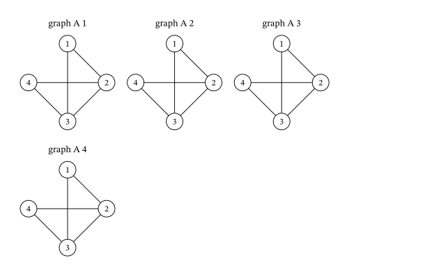
Isomorphic graphs that represent the same pattern of connections can look very different despite having the same underlying structure. The edges can be stretched and twisted. The graph can be rotated or flipped. For example, in Figure 12.41, each of the diagrams represents the same pattern of connections.

Four representations of the same graph are displayed. The graphs are labeled graph A 1, graph A 2, graph A 3, and graph A 4. In the first graph, the four vertices are connected by edges to resemble a square. The bottom-left and top-right vertices are connected using an edge. The other graph represents the same in different forms. — **Figure 12.41** Four Representations of the Same Graph

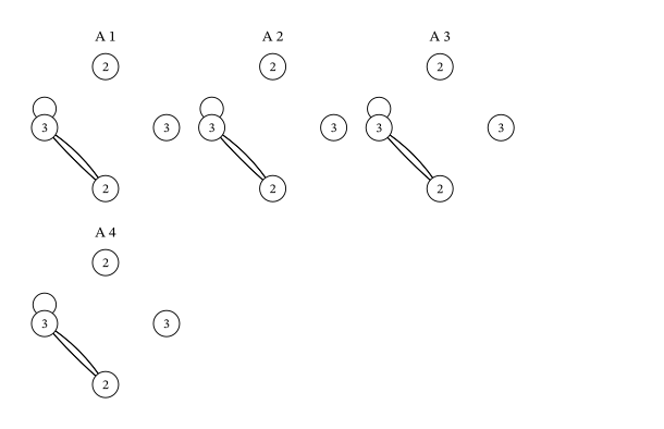
Looking at Figure 12.41, how can we know that these graphs are isomorphic? We will start by checking for any obvious differences. Each of the graphs in Figure 12.41 has four vertices and five edges; so, there are no differences there. Next, we will focus on the degrees of the vertices, which have been labeled in Figure 12.42.

As shown in Figure 12.42, each graph has two vertices of degree 2 and two vertices of degree 3; so, there are no differences there. Now, let’s check for cyclic subgraphs. These are highlighted in Figure 12.43.

Four representations of the same graph are displayed three times. In the first row, two squares, a quadrilateral, and a pentagon are highlighted. In the second row, a triangle and three other shapes are highlighted. In the third row, a triangle and three other shapes are highlighted. — **Figure 12.43** Graphs with the Same Cyclic Subgraphs

As shown in Figure 12.43, each graph has two triangles and one quadrilateral; so, no differences there either. It is beginning to look likely that these graphs are isomorphic, but we will have to look further to be sure.

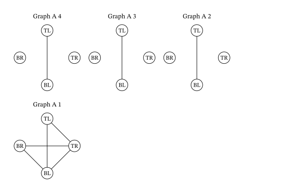
To know with certainty that these graphs are isomorphic, we need to confirm one of the two conditions from the definition of isomorphic graphs. With smaller graphs, you may be able to visualize how to stretch and twist one graph to get the other to see if condition 1 holds. Imagine the edges are stretchy and picture how to pull and twist one graph to form the other. If you can do this without breaking or adding any connections, then the graphs are really the same. Figure 12.44 demonstrates how to change graph A₄ to get A₃, graph A₃ to get A₂, and graph A₂ to get A₁.

Transformation of Graph A 4 to graph A 1 through graph A 3 and graph A 2. Graph A 4 has four vertices. It resembles a pentagon with a curved edge from the top-left vertex to the bottom-left vertex. The top-right vertex is moved to the center to obtain graph A 3. In graph A 3, the center vertex is moved to the top-left to obtain graph A 2. In graph A 2, the curved edge from the bottom-left vertex to the top-right vertex is shifted inside the graph to obtain graph A 1. In graph A 1, the four vertices are in four corners and they are connected using edges to resemble a square. A diagonal edge from the bottom-left vertex connects to the top-right vertex. — **Figure 12.44** Transforming Graphs

Now that we have used visual analysis to see that condition 1 holds for graphs A₁, A₂, A₃, and A₄ in Figure 12.43, we know that they are isomorphic. In Figure 12.44, one of the edges of graph A₄ crossed another edge of the graph. By transforming it into graph A₃, we have “untangled” it. Graphs that can be untangled are called planar graphs. The complete graph with five vertices is an example of a nonplanar graph-that means that, no matter how hard you try, you can’t untangle it. But, when you try to figure out if two graphs are the same, it can be helpful to untangle them as much as possible to make the similarities and differences more obvious.

Example 1 Identifying Isomorphic Graphs

Which of the three graphs in Figure 12.45 are isomorphic, if any? Justify your answer.

Figure 12.45 Three Similar Graphs

Step 1: Check for differences in number of vertices, number of edges, degrees of vertices, and types of cycles to see if an isomorphism is possible.

Vertices: They all have the same number of vertices, 4.
Edges: They all have the same number of edges, 4.
Degrees: Graph B₁ and Graph B₂ each have a vertex of degree 3, while Graph B₃ does not. So, Graph B₃ is not isomorphic to either of the other two graphs, but Graph B₁ and Graph B₂ could possibly be isomorphic.
Cycles: Focus on any cycles in Graph B₁ and Graph B₂. Each graph has a triangle as shown in Figure 12.46.

Figure 12.46 Cycles of Graph B₁ and Graph B₂

Step 2: If no differences were found and an isomorphism is possible, verify one of the conditions in the definition of isomorphic.

Since we were able to determine that Graph B₁ and Graph B₂ have no obvious differences, and they are relatively small graphs, we will attempt to transform one graph into the other, which would verify condition 1. Graph B₁ can be transformed into Graph B₂ without breaking or adding connections as shown in Figure 12.47. Begin by untangling graph B₁. Then rotate or flip as needed to see that the graphs match.

Figure 12.47 Transformation of Graph B₁

So, Graph B₁ and Graph B₂ have the same structure and are isomorphic.

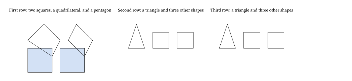
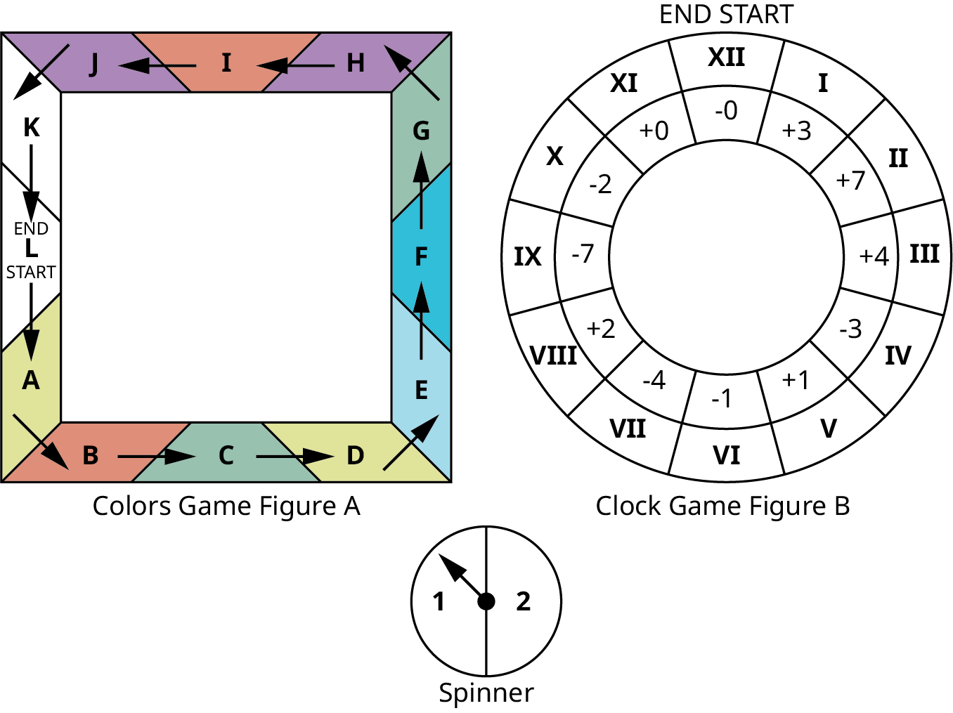
Have you ever noticed that many popular board games may look different but are really the same game? A good example is the many variations of the board game Monopoly®, which was submitted to the U.S. Patent Office in 1935. Although the rules have been revised a bit, a very similar game board is still in use today. There have been many versions of Monopoly over the years. Many have been stylized to reflect a popular theme, such as a show or sports team, while retaining the same game board structure. If we were to represent these different versions of the game using a graph, we would find that the graphs are isomorphic.. Let's analyze some game boards using graph theory to determine if they have the same structure despite having different appearances.

Two game boards and a spinner. The first game board is titled, Colors Game Figure A. It has 12 spaces arranged in a square. The spaces are as follows: A (yellow), B (red), C (green), D (yellow), E (blue), F (blue), G (green), H (purple), I (red), J (purple), K (white), L (white). Arrows show a path starting in space L and moving counterclockwise around the board to end in space L. The second game board is titled, Clock Game Figure B. It has 12 spaces arranged in a circle. The spaces are as follows: I (plus 3), II (plus 7), III (plus 4), IV (minus 3), V (plus 1), VI (minus 1), VII (minus 4), VIII (plus 2), IX (minus 7), X (minus 2), XI (plus 0), XII (minus 0). The space XII is indicated as the start and end space. A spinner has 2 sections labeled 1 and 2. — **Figure 12.48** Two Game Boards

Example 2 Deciding If Graphs are Isomorphic

A teacher uses games to teach her students about colors and numbers as shown in Figure 12.48.

In the Colors Game, shown in Figure A, each player begins in the space marked START and proceeds in a counterclockwise direction. On each turn, the player spins a spinner marked 1 and 2 and moves forward the number of spaces shown on the spinner. If the player lands on a space marked with any color other than white, the player must move forward or back to the other space of the same color. The first player to land in or pass the space marked END wins.

In the Clock Game, shown in Figure B, each player begins in the space marked START and proceeds in a clockwise direction. On each turn, the player spins a spinner marked 1 and 2 and moves forward the number of spaces shown on the spinner. In the same turn, the player must read the number in the space and move forward the number of spaces indicated by a positive value or backward the number of spaces indicated by a negative value. Then the turn ends. The first player to land in or pass the space marked END wins.

Draw a graph or multigraph to represent each game in which the vertices are the spaces and the edges represent the ability of a player to move between the spaces either by a spin or as dictated by a marked color or number. (We will ignore the direction of motion for simplicity.) Transform one of the graphs to show that it is isomorphic to the other and explain what this tells you about the games.

The graph representing the Clock Game can be transformed as shown in Figure 12.49 so that we can see that the graphs are isomorphic. There is a correspondence between their vertices in such a way that any adjacent pair in one graph corresponds to an adjacent pair in the other graph.

Figure 12.49 Graphs for Clock Game and Colors Game

This tells us that the games are essentially the same game with the same moves even though the games appear to be different.

People in Mathematics

Elizabeth Magie

Game designer, engineer, comedian, and political activist, Elizabeth Magie designed a game called “Landlord’s Game” to educate fellow citizens about the dangers of monopolies and the benefits of wealth redistribution through a land tax. Magie, whose father had campaigned with Abraham Lincoln, was a proponent of a land tax, an idea popularized by Henry George’s 1879 book, Progress and Poverty. She designed the game to be played by two sets of rules for comparison. In one version, the goal was to dominate opponents by creating monopolies, leaving one wealthy player standing in the end. In the other version, all the players were rewarded when a monopoly was created through a simulated land tax. She patented this game for the first time in 1904. Does the game board in Figure 12.50 look familiar?

Figure 12.50 Landlord’s Game PatentLandlord’s Game Patent (credit: "Landlord's Game Patent" Wikimedia Commons, Public Domain)

That’s right! A modified version of the game was obtained from friends by a man named Charles Darrow who renamed it Monopoly and sold to Parker Brothers. Parker Brothers later paid Magie $500 for the right to her patent on it. The property tax version was left behind, and the modern game of Monopoly was born. (Mary Pilon, Monopoly’s Lost Female Inventor, September 1, 2018, National Women’s History Museum, “Monopoly’s Lost Female Inventor,”

Identifying and Naming Isomorphisms

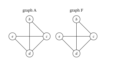
When two graphs are isomorphic, meaning they have the same structure, there is a correspondence between their vertices, which can be named by listing corresponding pairs of vertices. This list of corresponding pairs of vertices in such a way that any adjacent pair in one graph corresponds to an adjacent pair in the other graph is called an isomorphism. Consider the isomorphic graphs in Figure 12.38. In Figure 12.51, we could replace the labels Graph F with the labels from Graph A and have an identical graph, as in Figure 12.52.

Two graphs are labeled graph A and graph F. Graph A has four vertices: b, c, d, and e. The edges connect b c, c e, e d, d b, and d c. Graph F has four vertices: b, c, d, and e. The edges connect b c, c e, e d, d b, and d c. The vertices, g, h, i, and j are struck through and written as b, c, d, and e. — **Figure 12.52** Corresponding Vertices

So, we can identify an isomorphism between Graph A and Graph F by listing the corresponding pairs of vertices: b-g, c-h, d-i, and e-j. Notice that b is adjacent to c and g is adjacent to h. This must be the case since b corresponds to g and c corresponds to h. The same is true for other pairs of adjacent vertices.

An isomorphism between graphs is not necessarily unique. There can be more than one isomorphism between two graphs. We can see how to form a different isomorphism between Graph A and Graph F from Figure 12.33 by rotating Graph F clockwise and comparing the rotated version of F to Graph A as in YOUR TURN 12.13. Now, we can see that a second isomorphism exists, which has the correspondence: b-j, d-h, c-i, and e-g as shown in Figure 12.53.

Graph F is converted into graph A. Graph F has four vertices: g, h, i, and j. The edges connect g h, h j, j i, i g, and i h. Graph F is rotated 90 degrees clockwise. Graph F is rotated 180 degrees clockwise to obtain graph A. Graph A has four vertices: b, c, d, and e. The edges connect b c, c e, e d, d b, and d c. — **Figure 12.53** Transforming Graph F into Graph A

Example 4 Recognizing an Isomorphism

Determine whether Graphs G and S in Figure 12.56 are isomorphic. If not, explain how they are different. If so, name the isomorphism.

Figure 12.56 Graph G and Graph S

Step 1: Check for any differences.

Vertices: Graphs G and S each have six vertices.
Edges: Graphs G and S each have six edges.
Degrees: Each graph also has two vertices of degree 1, two vertices of degree 2, and two vertices of degree 3.
Cycles: From Figure 12.57, we can see that Graph G contains a quadrilateral cycle (b, f, d, c) but Graph S has no quadrilaterals. Also, Graph S contains a triangle cycle (m, r, o) but Graph G has no triangles. This means that the graphs are not isomorphic.

Figure 12.57 Comparing Subgraphs

Step 2: This step is not necessary because we now know Graphs G and S are not isomorphic.

Complementary Graphs

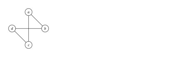
Suppose that you are a camp counselor at Camp Woebegone and you are holding a camp Olympics with four events. The campers have signed up for the events. You drew a graph in Figure 12.58 to help you visualize which events have campers in common.

A graph with four vertices. The vertices are labeled, a, b, c, and d. The edges connect a b, b d, d c, and c a. — **Figure 12.58** Graph of Events with Campers in Common

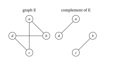
Graph E in Figure 12.58 shows that some of the same campers will be in events a and b, as well as b and d, c and d, and a and c. What do you think the graph would look like that represented the events that do not have campers in common? It would have the same vertices, but any pair of adjacent edges in Graph E, would not be adjacent in the new graph, and vice versa. This is called a complementary graph, as shown in Figure 12.59. Two graphs are complementary if they have the same set of vertices, but any vertices that are adjacent in one, are not adjacent in the other. In this case, we can say that one graph is the complement of the other.

Two graphs: graph E and complement of E. Graph E has four vertices: a, b, c, and d. The edges connect a b, b d, d c, and c a. The complement of E has four vertices: a, b, c, and d. The edges connect a d, and b c. — **Figure 12.59** Graphs of Camp Olympics

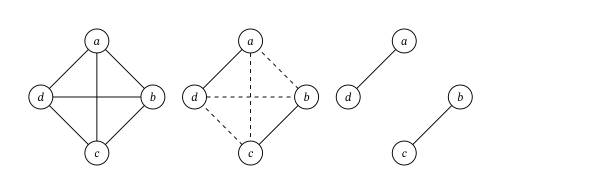
One way to find the complement of a graph is to draw the complete graph with the same number of vertices and remove all the edges that were in the original graph. Let’s say you wanted to find the complement of Graph E from Figure 12.59, and you didn’t already know it was Graph F. You could start with the complete graph with four vertices and remove the edges that are in Graph E as shown in Figure 12.60.

Three graphs. The first graph has four vertices: a, b, c, and d. The edges connect a b, b d, d c, c a, a d, and b c. The second graph has four vertices: a, b, c, and d. The edges connecting a b, b d, d c, and c a are struck through. The edges connect a d and c b. The third graph has four vertices: a, b, c, and d. The edges connect a d and c b. — **Figure 12.60** Use Complete Graph to Find Complement

Example 5 Finding a Complement

A particular high school has end-of-course exams in (E3) English 3, (E4) English 4, (M) Advanced Math, (C) Calculus, (W) World History, (U) U.S. History, (B) Biology, and (P) Physics. No English 3 students are taking English 4, World History, or Biology; no English 4 students are also in Calculus, Advanced Math, U.S. History, or Physics; no Physics students are also taking Advanced Math; No World History students are also taking U.S. History; and no Advanced Math students are also taking Calculus.

Create a graph in which the vertices represent the exams, and an edge between a pair of vertices indicates that there are no students taking both exams.
Find the complement of the graph in part 1.
Explain what the graph in part 2 represents.

In Figure 12.61, we have drawn a vertex for each exam and edges between any vertices that have no students in common.
Figure 12.61 Graph of Exams with No Students in Common
One way to get the complement of the graph in Figure 12.61 is to draw a complete graph with the same number of vertices and remove the edges they have in common as shown in Figure 12.62.
Figure 12.62 Remove Unwanted Edges from Complete Graph
The final graph of the complement is in Figure 12.63.
Figure 12.63 Graph of Exams with Students in Common
In the graph in Figure 12.63, the vertices are still the exams, and a pair of adjacent vertices represents a pair of exams that have students in common.

When two graphs are really the same graph, they have the same missing edges. So, when two graphs have a lot of edges, it may actually be easier to determine if they are isomorphic by looking at which edges are missing rather than which edges are included. In other words, we can determine if two graphs are isomorphic by checking if their complements are isomorphic.

Example 6 Using a Complement to Find an Isomorphism

Use Figure 12.64 to answer each question.

Figure 12.64 Graph K

Find the complement of Graph K.
Identify an isomorphism between the complement of Graph K from part 1, and the complement of Graph H in YOUR TURN 12.17.
Confirm that the correspondence between the vertices you found in part 2 also gives an isomorphism between Graph H from YOUR TURN 12.17, and Graph K from Figure 12.64.

The complement of Graph K can be found by removing the edges of Graph K from a complete graph with the same vertices as shown in Figure 12.65.
Figure 12.65 Find Complement of Graph K
An isomorphism between the complement of Graph K and the complement of Graph H is A-M, C-L, E-N, B-O, and D-P, which is confirmed by transforming the complement of Graph K in Figure 12.66.
Figure 12.66 Isomorphism between Complements of K and H
Figure 12.67 shows how Graph K can be transformed into Graph H to confirm that the correspondence is A-M, C-L, E-N, B-O, and D-P also gives an isomorphism between Graph K and Graph H.
Figure 12.67 Isomorphism between K and H

This means we now have three conditions that guarantee two graphs are isomorphic.

First Way: One graph can be transformed into the other without breaking existing connections or adding new ones.

Second Way: There is a correspondence between their vertices in such a way that any adjacent pair in one graph corresponds to an adjacent pair in the other graph.

Third Way: Their complements are isomorphic.

If any one of these statements is true, then they are all true. If any one of these statements is false, then they are all false.

Work It Out

Here is an activity you can do with a few of your classmates that will build your graph comparison skills.

Step 1: Draw a planar graph with the following characteristics: exactly five vertices, one vertex of degree four, at least two vertices of degree three, and exactly eight edges. Give names to the vertices. Make sure you do not use the same letters or numbers to label your vertices as your classmates do.

Step 2: Analyze your graph. What is the degree of each vertex? Does your graph have any cyclic subgraphs? If so, list them and indicate their sizes.

Step 3: Draw and analyze the complement of your graph. How many edges and vertices does it have? What is the degree of each vertex? Does the complementary graph have any cyclic subgraphs? If so, list them and indicate their sizes.

Step 4: Compare your graphs to each of your classmates’ graphs. Does your graph have the same number of edges and vertices as the graph of your classmate? Does your graph have the same size cyclic subgraphs as the graph of your classmate? How does the complement of your graph compare to the complement of the graph of your classmate? Determine if your graph is isomorphic to your classmates’ graph. If so, give a correspondence that demonstrates the isomorphism. If not, explain how you know.

Key Terms

isomorphic
isomorphism
planar
nonplanar
complement
complementary

Key Concepts

Two graphs are isomorphic if they have the same structure.
When graphs are relatively small, we can use visual inspection to identify an isomorphism by transforming one graph into another without breaking connections or adding new ones.
An isomorphism between two graphs preserves adjacency.
If two graphs differ in number of vertices, number of edges, degrees of vertices, or types of subgraphs, they cannot be isomorphic.
When the complements of two graphs are isomorphic, so are the graphs themselves.

Videos

Determine If Two Graphs Are Isomorphic and Identify the Isomorphism

Adapted from Contemporary Mathematics by OpenStax (openstax.org), licensed under CC BY-NC-SA 4.0. Changes were made. License: CC-BY-NC-SA-4.0.