
12.4 Navigating Graphs
Learning Objectives
After completing this section, you should be able to:
- Describe and identify walks, trails, paths, and circuits.
- Solve application problems using walks, trails, paths, and circuits.
- Identify the chromatic number of a graph.
- Describe the Four-Color Problem.
- Solve applications using graph colorings.
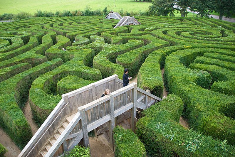
Now that we know the basic parts of graphs and we can distinguish one graph from another, it is time to really put our graphs to work for us. Many applications of graph theory involve navigating through a graph very much like you would navigate through a maze. Imagine that you are at the entrance to a maze. Your goal is to get from one point to another as efficiently as possible. Maybe there are treasures hidden along the way that make straying from the shortest path worthwhile, or maybe you just need to get to the end fast. Either way, you definitely want to avoid any wrong turns that would cause unnecessary backtracking. Luckily, graph theory is here to help!
Walks
Suppose Figure 12.69 is a maze you want to solve. You want to get from the start to the end.
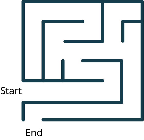
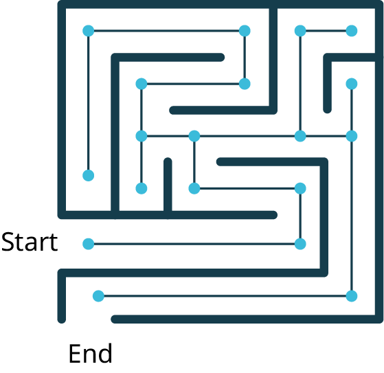
You can approach this task any way you want. The only rule is that you can’t climb over the wall. To put this in the context of graph theory, let’s imagine that at every intersection and every turn, there is a vertex. The edges that join the vertices must stay within the walls. The graph within the maze would look like Figure 12.70.
One approach to solving a maze is to just start walking. It is not the most efficient approach. You might cross through the same intersection twice. You might backtrack a bit. It’s okay. We are just out for a walk. It might look something like the black sequence of vertices and edges in Figure 12.71.
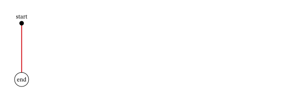
This type of sequence of adjacent vertices and edges is actually called a walk (or directed walk) in graph theory too!
A walk can be identified by naming the sequence of its vertices (or by naming the sequence of its edges if those are labeled). Let’s take the graph out of the context of the maze and give each vertex a name and each edge of the walk a direction as in Figure 12.72.
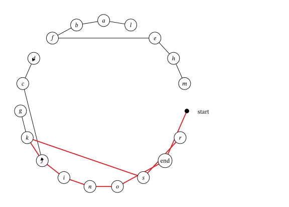
The name of this walk from p to r is p → q → o → n → i → j → c → d → c → j → k → s → r. When a particular edge on our graph was traveled in both directions, it had arrows in both directions and the letters of vertices that were visited more than once had to be repeated in the name of the walk.
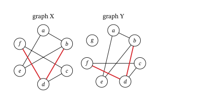
The highlighted edges Graph Y in Figure 12.73 represent a walk between f and b. The highlighted edges in Graph X do not represent a walk between f and b, because there is a turn at a point that is not a vertex. This is like climbing over a wall when you are walking through a maze. Another way of saying this is that b → d → f is not a walk, because there is no edge between b and d.
Paths and Trails
A walk is the most basic way of navigating a graph because it has no restrictions except staying on the graph. When there are restrictions on which vertices or edges we can visit, we will call the walk by a different name. For example, if we want to find a walk that avoids travelling the same edge twice, we will say we want to find a trail (or directed trail). If we want to find a walk that avoids visiting the same vertex twice, we will say, we want to find a path (or directed path).
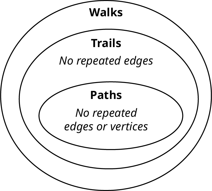
Walks, trails, and paths are all related.
- All paths are trails, but trails that visit the same vertex twice are not paths.
- All trails are walks, but walks in which an edge is visited twice would not be trails.
We can visualize the relationship as in Figure 12.78.
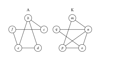
Let’s practice identifying walks, trails, and paths using the graphs in Figure 12.79.
Circuits
In many applications of graph theory, such as creating efficient delivery routes, beginning and ending at the same location is a requirement. When a walk, path, or trail end at the same location or vertex they began, we call it closed. Otherwise, we call it open (does not begin and end at the same location or vertex). Some examples of closed walks, closed trails, and closed paths are given in in the following table.
| DESCRIPTION | EXAMPLE | CHARACTERISTICS |
|---|---|---|
| A closed walk is a walk that begins and ends at the same vertex. | d → f → b → c → f → d | Alternating sequence of vertices and edges Begins and ends at the same vertex |
| A closed trail is a trail that begins and ends at the same vertex. It is commonly called a circuit. | d → f → b → c → f → e → d | No repeated edges Begins and ends at the same vertex |
| A closed path is a path that begins and ends at the same vertex. It is also referred to as a directed cycle because it travels through a cyclic subgraph. | d → f → b → c → d | No repeated edges or vertices Begins and ends at the same vertex |
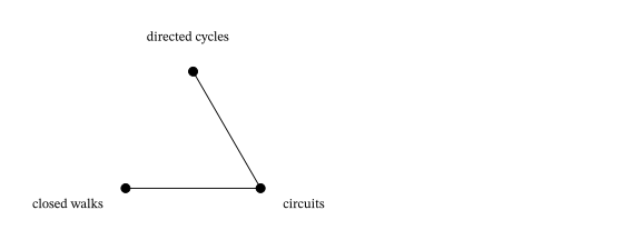
Since walks, trails, and paths are all related, closed walks, circuits, and directed cycles are related too.
- All circuits are closed walks, but closed walks that visit the same edge twice are not circuits.
- All directed cycles are circuits, but circuits in which a vertex is visited twice are not directed cycles.
We can visualize the relationship as in Figure 12.84.
The same circuit can be named using any of its vertices as a starting point. For example, the circuit d → f → b → c → d can also be referred to in the following ways.
a → b → c → d → a is the same as
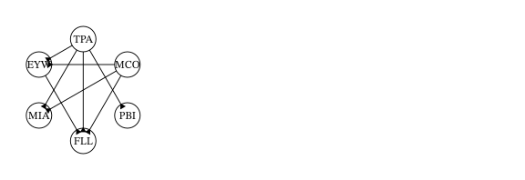
Let’s practice working with closed walks, circuits (closed trails), and directed cycles (closed paths). In the graph in Figure 12.85, the vertices are major central and south Florida airports. The edges are direct flights between them.
Graph Colorings
In this section so far, we have looked at how to navigate graphs by proceeding from one vertex to another in a sequence that does not skip any vertices, but in some applications we may want to skip vertices. Remember the camp Olympics at Camp Woebegone in Comparing Graphs? You were planning a camp Olympics with four events. The campers signed up for the events. You drew a graph to help you visualize which events have campers in common. The vertices of Graph E in Figure 12.87 represent the events and adjacent vertices indicate that there are campers who are participating in both.
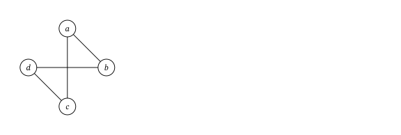
In this case, we do NOT want events represented by two adjacent vertices to occur in the same timeslot, because that would prevent the campers who wanted to participate in both from doing so. We can use the graph in Figure 12.87 to count the timeslots we need so there are no conflicts. Let’s assign each timeslot a different color. We could categorize events that happen at 1 pm as Red; 2 pm, Purple; 3 pm, Blue; and 4 pm, Green. Then assign different colors to any pair of adjacent vertices to ensure that the events they represent do not end up in the same timeslot. Figure 12.88 shows several of the ways to do this while obeying the rule that no pair of adjacent vertices can be the same color.
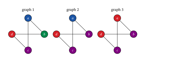
In Figure 12.88, the graphs with vertices colored so that no adjacent vertices are the same color are called graph colorings. Notice that Graph 3 has the fewest colors, which means it shows us how to have the fewest number of timeslots. The events marked in red, a and d, can be held at the same time because they are not adjacent and do not have conflicts. Also, the events marked in purple, b and c, can be held at the same time. We would not need green or blue timeslots at all!
A graph that uses colors is called an -coloring. The smallest number of colors needed to color a particular graph is called its chromatic number.
Graph colorings can be used in many applications like the scheduling scenario at camp Woebegone. Let's look at how they work in more detail. Figure 12.89 shows two different colorings of a particular graph. Coloring A is called a four-coloring, because it uses four colors, red (R), green (G), blue (B), and purple (P). Coloring B is called a three-coloring because it uses three. The colors allow us to visually subdivide the graphs into groups. The only rule is that adjacent vertices are different colors so that they are in different groups.
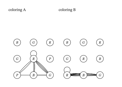
It turns out that a three-coloring is the best we can do with the graph in Figure 12.89. No matter how many different patterns you try with only two colors, you will never find one in which the adjacent vertices are always different colors. In other words, the graph has a chromatic number of three. For large graphs, computer assistance is usually required to find the chromatic numbers. There is no formula for finding the chromatic number of a graph, but there are some facts that are helpful in Table 12.5.
| Fact | Example |
|---|---|
| Recall that planar graphs are untangled; that is, they can be drawn on a flat surface so that no two edges are crossing. If a graph is planar, it can be colored with four colors or possibly fewer. | |
| Each vertex in a complete graph is adjacent to every other vertex forcing us to color them all different colors.The chromatic number of a complete graph is the same as the number of vertices. | |
| If a graph has a clique, a complete subgraph, then each vertex in the clique must have a different color and the vertices outside the clique may or may not have even more colors. The chromatic number of a graph is at least the number of vertices in its biggest clique. |
Creating Colorings to Solve Problems
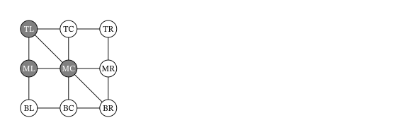
Let’s see how these facts can help us color the graph in Figure 12.90.
- Since the graph is planar, the chromatic number is no more than four.
- The graph is not complete, but it has complete subgraphs of three vertices. In other words, it has triangles like the one shown with blue vertices in Figure 12.90. This means that the chromatic number is at least three.
We know we can color this graph in three or four colors. It is usually best to start by coloring the vertex of highest degree as shown in Figure 12.91. In this case, we used red (R). The color is not important.
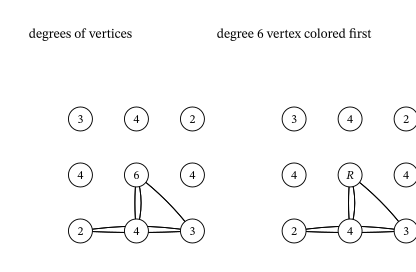
We want to color as many of the vertices the same color as possible; so, we look at all the vertices that are not adjacent to the red vertex and begin to color them, red starting with the one among them of highest degree. Since the only vertices that are not adjacent are both degree 2, choose either one and color it red as shown in Figure 12.92.
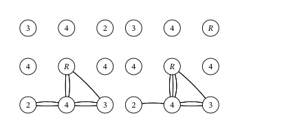
Now, there is only one vertex left that is not adjacent to a red; so, color it red. Of the remaining vertices, the highest degree is four; so, color one of the vertices of degree four in a different color. These two steps are shown in Figure 12.93.
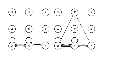
Repeat the same procedure. There are three remaining vertices that are not adjacent to a blue. Color as many blue as possible, with priority going to vertices of higher degree as shown in Figure 12.94.
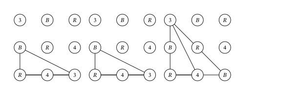
All the remaining vertices are adjacent to blue. So, it is time to repeat the procedure with another color as shown in Figure 12.95.
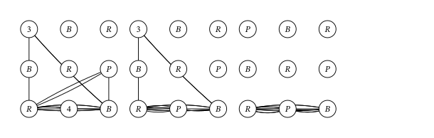
All the vertices are now colored with a three-coloring so we know the chromatic number is at most three, but we knew the chromatic number was at least three because the graph has a triangle. So, we are now certain it is exactly three.
Suppose the vertices of the graph in Figure 12.96 represented the nine events in the Camp Woebegone Olympics, and edges join any events that have campers in common, but nonadjacent vertices do not.
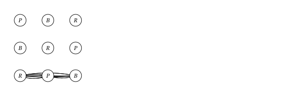
Any vertices of the same color are nonadjacent; so, they have no conflicts. Since this graph is a three-coloring, all nine events could be scheduled in just three timeslots!
The Four Color Problem
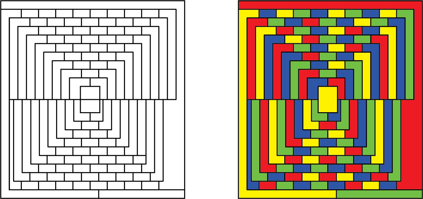
The idea of coloring graphs to solve problems was inspired by one of the most famous problems in mathematics, the “four color problem.” The idea was that, no matter how complicated a map might be, only four colors were needed to color the map so that no two regions that shared a boundary would be the same color. For many years, everyone suspected this to be true, because no one could create a map that needed more than four colors, but they couldn’t prove it was true in general. Finally, graphs were used to solve the problem!
We saw how maps can be represented as graphs in Graph Basics. Figure 12.99 from Example 4 in Section 12.1 shows a map of the midwestern region of the United States.
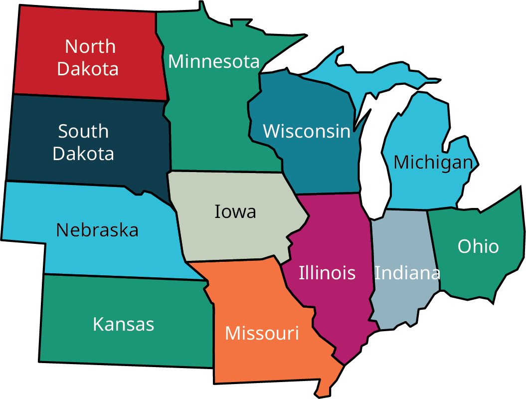
Figure 12.100 shows how this map can be associated with a graph in which each vertex represents a state and each edge indicates the states that share a common boundary. Figure 12.101 shows the final graph.
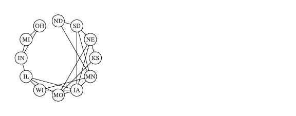
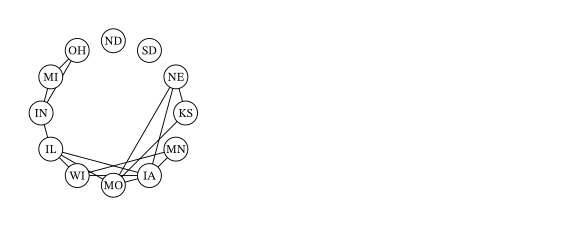
Notice that the graph representing the common boundaries between midwestern states is planar, meaning that it can be drawn on a flat surface without edges crossing. As we have seen, any planar graph has a chromatic number of four or less. This very well-known fact is called the Four-Color Theorem, or Four-Color Map Theorem.
Key Terms
- walk (directed walk)
- trail (directed trail)
- path (directed path)
- closed
- open
- closed walk
- circuit (closed trail)
- directed cycle (closed path)
- coloring (graph coloring)
- -coloring
- chromatic number
Key Concepts
- Walks, trails, and paths are ways to navigate through a graph using a sequence of connected vertices and edges.
- Closed walks, circuits, and directed cycles are ways to navigate from a vertex on a graph and return to the same vertex.
- Colorings are a way to organize the vertices of a graph into groups so that no two members of a group are adjacent.
- Maps can be represented with planar graphs, which can always be colored using four colors or fewer.
Videos
- Walks, Trails, and Paths in Graph Theory
- Closed Walks, Closed Trails (Circuits), and Closed Paths (Directed Cycles) in Graph Theory
- Coloring Graphs Part 1: Coloring and Identifying Chromatic Number
- The Four Color Map Theorem – Numberphile
- Coloring Graphs Part 2: Coloring Maps and the Four Color Problem
- Neil deGrasse Tyson Explains the Möbius Strip
Adapted from Contemporary Mathematics by OpenStax (openstax.org), licensed under CC BY-NC-SA 4.0. Changes were made. License: CC-BY-NC-SA-4.0.