
12.2 Graph Structures

Learning Objectives
After completing this section, you should be able to:
- Describe and interpret relationships in graphs.
- Model relationships with graphs.
Graph theory is used in neuroscience to study how different parts of the brain connect. Neurobiologists use functional magnetic resonance imaging (fMRI) to measure levels of blood in different parts of the brain, called nodes. When nodes are active at the same time, it suggests there is a functional connection between them so they form a network. This network can be represented as a graph where the vertices are the nodes and the functional connections are the edges between them. (Mikey Taylor, "Graph Theory & Machine Learning in Neuroscience," Medium.com, June 24, 2020.
Importance of the Degrees of Vertices
One reason scientists study these networks is to determine how successful the communication within a network continues to be when it experiences failures in nodes and connections. Graphs can be used to study the resilience of these networks. (Mikey Taylor, "Graph Theory & Machine Learning in Neuroscience," Medium.com, June 24, 2020)
Relating the Number of Edges to the Degrees of Vertices
In the applications of graph theory to neuroscience and sociology in Example 1 and YOUR TURN 12.6, there was a correlation between the degrees of vertices and the resilience of a network. Researchers in many fields have also observed a direct relationship between the number of edges in a graph and the degrees of the vertices. To begin to understand this relationship, consider a graph with five vertices and zero edges as in Figure 12.18.
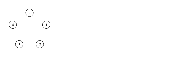
Instead of being marked with a name, each vertex in Figure 12.18 is marked with its degree. In this case, all of the degrees are 0 so the sum of the degrees is also zero. Suppose that we add an edge between any two existing vertices and indicate the degrees of the vertices. This gives us a graph with five vertices and one edge like the graph in Figure 12.19.
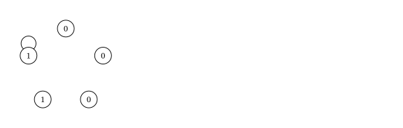
Note that the degrees of two vertices increased, each by 1. So, the sum of the degrees is now 2. Suppose that we continue in this way, adding one edge at a time and making note of the number of edges and the sum of the degrees of the vertices as in Figure 12.20.
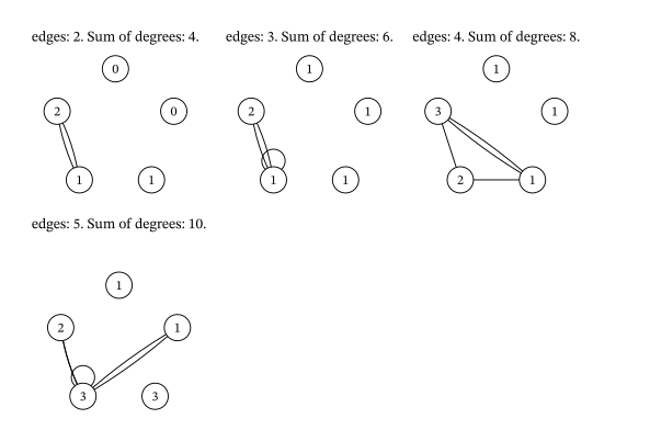
Figure 12.20 demonstrates a characteristic that is true of all graphs of any shape or size. When the number of edges is increased by one, the sum of the degrees increases by two. This happens because each edge has two ends and each end increases the degree of one vertex by one unit. As a result, the sum of the degrees of the vertices on any graph is always twice the number of edges. This relationship is known as the Sum of Degrees Theorem.
Completeness
Suppose that there were five strangers in a room, A, B, C, D, and E, and each one would be introduced to each of the others. How many introductions are necessary? One way to begin to answer this question is to draw a graph with each vertex representing an individual in the room and each edge representing an introduction as in Figure 12.22.
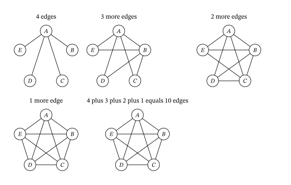
Let’s approach the problem by thinking about how many new people Person A would meet, then Person B, and so on, making sure not to repeat any introductions. The first graph in Figure 12.22 shows Person A meeting Persons B, C, D, and E, for a total of 4 introductions. The next graph shows that Person B still has to meet Persons C, D, and E, for a total of 3 more introductions. The next graph shows that Person C still has to meet Persons D and E, which is 2 more introductions. The next graph shows that Person D only remains to meet Person E, which is 1 more introduction. The final graph has edges representing 10 introductions. The last graph is an example of a complete graph because each pair of vertices is joined by an edge. Another way of saying this is that the graph is complete because each vertex is adjacent to every other vertex.Figure 12.23 shows complete graphs with three, four, five, and six vertices.
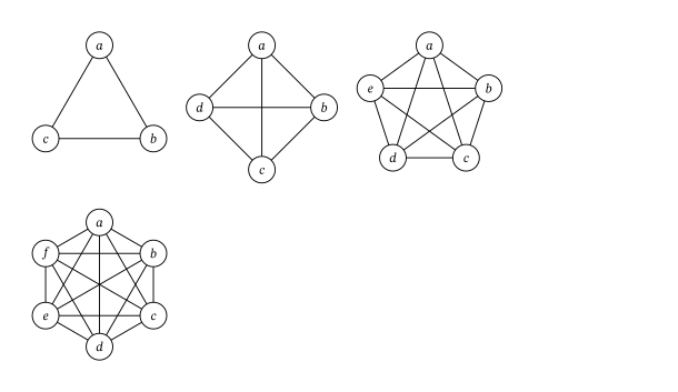
Suppose we want to know the number of introductions necessary in a room with six people. This would be represented by a complete graph with six vertices, and the total number of introductions would be , the number of edges in the graph. In fact, you can always find the number of introductions in a room with people by adding all the whole numbers from 1 to .
Suppose that we want to determine how many introductions are necessary in a room with 500 strangers. In other words, suppose that we want to determine the number of edges in a complete graph with 500 vertices. Adding up all the numbers from 1 to 499 could take a long time! In the next example, we use the Sum of Degrees Theorem to make the problem more manageable.
Now we have a shorter way to calculate the number of introductions in a room with strangers, and the number of edges on a complete graph with vertices. Let’s update our formula.
Subgraphs
Sometimes a graph is a part of a larger graph. For example, the graph of South Florida Airports from Figure 12.7 is part of a larger graph that includes Orlando International Airport in Central Florida, which is shown in Figure 12.24
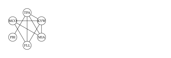
The graph in Figure 12.24 includes an additional vertex, MCO, and additional edges shown with dashed lines. The graph of direct flights between South Florida airports from Figure 12.7 is called a subgraph of the graph that also includes direct flights between Orlando and the same South Florida airports in Figure 12.24. In general terms, if Graph B consists entirely of a set of edges and vertices from a larger Graph A, then B is called a subgraph of A.
Identifying and Naming Cycles

When you think of a cycle in everyday life, you probably think of something that begins and ends the same way. For example, the water cycle (Figure 12.26) begins with water in a lake or ocean, which evaporates into water vapor, condenses into clouds, and then returns to earth as rain or some other form of precipitation that settles into lakes or oceans. A cycle in graph theory is similar in that it begins and ends in the same way: It is a series of connected edges that begin and end at the same vertex but otherwise never repeat any vertices.
In a cycle, there are always the same number of vertices as edges, and all vertices must be of degree 2. Cycles are often referred to by the number of vertices. For example, a cycle with 5 vertices can be called a 5-cycle. Cycles can also be named after polygons based on the number of edges. For example a 5-cycle is also called a pentagon. Table 12.1 lists these names for cycles of size 3 through size 10.
| Cycle Category | Number of Edges | Example |
|---|---|---|
| triangle | 3 | |
| quadrilateral | 4 | |
| pentagon | 5 | |
| hexagon | 6 | |
| heptagon | 7 | |
| octagon | 8 | |
| nonagon | 9 | |
| decagon | 10 |
There are many more polygon names, including a megagon that has a million edges and a googolgon that has edges, but usually we just say -gon when the number is past 10. For example, a cycle with 11 edges could be called an 11-gon.
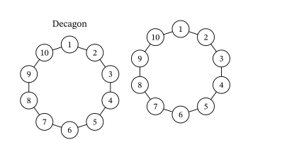
Notice that the 10-cycle, or decagon, appears to cross over itself in Table 12.1. Remember, graphs can be drawn differently but represent the same connections. In Figure 12.27, the same decagon is transformed into a graph that does not appear to overlap itself. We have done this without changing any of the connections so both diagrams represent the same relationships, and both diagrams are considered decagons.
Cyclic Subgraphs and Cliques
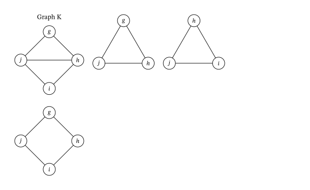
When cycles appear as subgraphs within a larger graph, they are called cyclic subgraphs. Cyclic subgraphs are named by listing their vertices sequentially. The vertex where you begin is not important. Graph K in Figure 12.28 has two triangle cycles (g, h, j) and (h, i, j), and one quadrilateral cycle (g, h, i, j).
We have seen that sociologists use graphs to study the structures of social networks. In sociology, there is a principle known as Triadic Closure. It says that if two individuals in a social network have a friend in common, then it is more likely those two individuals will become friends too. Sociologists refer to this as an open triad becoming a closed triad. This concept can be visualized as graphs in Figure 12.30. (Chakraborty, Dutta, Mondal, and Nath, "Application of Graph Theory in Social Media, International Journal of Computer Sciences and Engineering, 6(10):722-729) In the open triad in Figure 12.30, person a and person b each has a friendship with person c. In the closed triad, person a and person b have also developed a friendship. Notice that the graph representing the closed triad is a three-cycle, or a triangle, in graph theory terms.
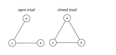
Another topic of interest to sociologists, as well as computer scientists and scientists in many fields, is the concept of a clique. In a social group, a clique is a subgroup who are all friends. A triad is an example of a clique with three people, but there can be cliques of any size. In graph theory, a clique is a complete subgraph.
Three-Cycles in Complete Graphs
Just as complete graphs have a predictable number of edges, complete graphs have a predictable number of cyclic subgraphs. Let’s look at the three-cycles within complete graphs with up to six vertices, which are shown in Figure 12.31.
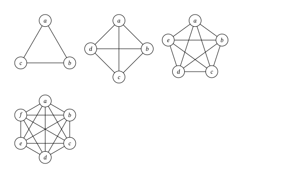
Let's list the names of all the triangles in each graph. Since every pair of vertices is adjacent, any three vertices on a complete graph form a triangle. There is only one triangle in the complete graph with three vertices, (a, b, c). For the rest of the graphs, it is important that we take an organized approach. Start with the vertex that is first alphabetically, listing any triangles that include that vertex also in alphabetical order. Then, proceed to the next vertex in the alphabet, and list any triangles that include that vertex, except those that are already listed. Keep going in this way as shown in Table 12.2.
| Complete Graph With: | 3 Vertices | 4 Vertices | 5 Vertices | 6 Vertices |
|---|---|---|---|---|
| All a triangles | (a, b, c) | (a, b, c), (a, b, d), (a, c, d) | (a, b, c), (a, b, d), (a, b, e) (a, c, d), (a, c, e) (a, d, e) | (a, b, c), (a, b, d), (a, b, e), (a, b, f) (a, c, d), (a, c, e), (a, c, f) (a, d, e), (a, d, f) (a, e, f) |
| Other b triangles | None | (b, c, d) | (b, c, d), (b, c, e), (b, d, e) | (b, c, d), (b, c, e), (b, c, f) (b, d, e), (b, d, f) (b, e, f) |
| Other c triangles | None | None | (c, d, e) | (c, d, e), (c, d, f) (c, e, f) |
| Other d triangles | None | None | None | (d, e, f) |
| Total | 1 |
Look at the last row in Table 12.2. Do you see a pattern emerge for counting triangles in a complete graph? Without drawing a complete graph with 7 vertices, we can predict that it will have triangles inside it. This pattern also appears in a famous diagram known to Western mathematicians as "Pascal’s Triangle." Figure 12.32 displays the first 11 rows of Pascal’s Triangle. Row 0 of Pascal’s Triangle only has the number 1 in it. The first and last entries in each of the other rows are also 1s. Otherwise, all the entries are formed by adding two entries from the previous row. For example, in row 6, entry 1 is 6, which was found by adding 1 and the 5 from the previous row, and entry 2 is 15, which was found by adding the 5 and the 10 from the previous row, as shown in Table 12.2.
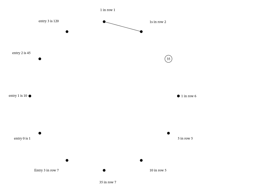
If we begin to list the third entries in each row of Pascal's triangle from the top down, we see 1, 4, 10, 20, 35, and so on. Notice that these values are exactly the number of triangles in a complete graph of sizes 3, 4, 5, 6, and 7, respectively. Specifically, entry 3 in row 7 is 35, the number of triangles in a complete graph of size 7. Let's practice using Pascal’s triangle to find the number of triangles in a complete graph of a particular size.
STEPS TO FIND THE NUMBER OF TRIANGLES IN A COMPLETE GRAPH OF SIZE n
Step 1 Calculate the entries in row n of Pascal's Triangle using sums of pairs of entries in previous rows as needed.
Step 2 The number of triangles is entry 3 in row n. Remember to count the entries 0, 1, 2, and 3, from left to right.
Key Terms
- complete
- subgraph
- cycle
- cyclic subgraph
- clique
Key Concepts
- The sum of the degrees of the vertices in a graph is twice the number of edges.
- In a complete graph every pair of vertices is adjacent.
- A subgraph is part of a larger graph.
- Cycles are a sequence of connected vertices that begin and end at the same vertex but never visit any vertex twice.
Formulas
For the Sum of Degrees Theorem, or
The number of edges in a complete graph with vertices is the sum of the whole numbers from 1 to , .
The number of edges in a complete graph with vertices is .
Videos
Adapted from Contemporary Mathematics by OpenStax (openstax.org), licensed under CC BY-NC-SA 4.0. Changes were made. License: CC-BY-NC-SA-4.0.