
2.4 Functions as Mathematical Models
The Shape of the Graph
Creating a good model for a situation often begins with deciding what kind of function to use. An appropriate model can depend on very qualitative considerations, such as the general shape of the graph. What sort of function has the right shape to describe the process we want to model? Should it be increasing or decreasing, or some combination of both? Is the slope constant or is it changing?
In Examples Example and Example, we investigate how the shape of a graph illustrates the nature of the process it models.
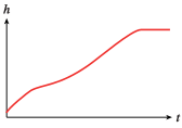
Erin walks from her home to a convenience store, where she buys some cat food, and then walks back home. Sketch a possible graph of her distance from home as a function of time.
The graph of Erin's distance from home is
_____
A graph is also shown below.
Alternate graph:
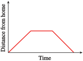
Erin walks from her home to a convenience store, where she buys some cat food, and then walks back home. Sketch a possible graph of her distance from home as a function of time.
The graphs in Example are piecewise linear, because Forrest traveled at a constant rate in each segment. In addition to choosing a graph that is increasing, decreasing, or constant to model a process, we can consider graphs that bend upward or downward. The bend is called the concavity of the graph.
A graph that bends upward is called concave up, and one that bends down is concave down.
A graph whose slopes decrease for increasing is called
_____
A graph whose slopes decrease for increasing is called concave down.
A graph whose slopes decrease for increasing is called
- increasing.
- decreasing.
- concave up.
- concave down.
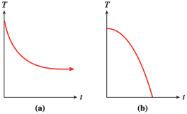
Francine bought a cup of cocoa at the cafeteria. The cocoa cooled off rapidly at first, and then gradually approached room temperature. Which graph more accurately reflects the temperature of the cocoa as a function of time? _____
Explain why. (Select all that apply.)
- The graph has a steep negative slope at first, corresponding to an initial rapid drop in the temperature of the cocoa. _____
- The graph becomes closer to a horizontal line, corresponding to the cocoa approaching room temperature._____
- The graph has a slight negative slope at first, corresponding to an initial rapid drop in the temperature of the cocoa. _____
- The graph becomes grows steeper and steeper, corresponding to the cocoa approaching room temperature. _____
Is the graph you chose concave up or concave down? _____
Graph (a): The graph has a steep negative slope at first, corresponding to an initial rapid drop in the temperature of the cocoa. The graph becomes closer to a horizontal line, corresponding to the cocoa approaching room temperature. The graph is concave up.
Francine bought a cup of cocoa at the cafeteria. The cocoa cooled off rapidly at first, and then gradually approached room temperature. Which graph more accurately reflects the temperature of the cocoa as a function of time? Explain why. Is the graph you chose concave up or concave down?
Graph (a): The graph has a steep negative slope at first, corresponding to an initial rapid drop in the temperature of the cocoa. The graph becomes closer to a horizontal line, corresponding to the cocoa approaching room temperature. The graph is concave up.
How can you tell from a table of values whether a function is concave up or concave down?
_____
How can you tell from a table of values whether a function is concave up or concave down?
Using the Basic Functions as Models
In Section 1.5 we considered some situations that can be modeled by linear functions. In this section, we consider some situations that can be modeled by the other basic functions. Example illustrates an application of the function .
Which graph is concave down wherever it is defined?
_____
The graph of is concave down.
Which graph is concave down wherever it is defined?
The ultraviolet index (UVI) is issued by the National Weather Service as a forecast of the amount of ultraviolet radiation expected to reach Earth around noon on a given day. The data show how much exposure to the sun people can take before risking sunburn.
| UVI | ||||||||
|---|---|---|---|---|---|---|---|---|
| Minutes to burn (more sensitive) | ||||||||
| Minutes to burn (less sensitive) |
- Plot , the minutes to burn, against , the UVI, to obtain two graphs, one for people who are more sensitive to sunburn, and another for people less sensitive to sunburn. Which of the basic functions do your graphs most resemble?
_____ - For each graph, find a value of so that fits the data.
More sensitive: _____
Less sensitive: _____
- The graphs are shown below. The shapes of the graphs resemble .
- More sensitive: , Less sensitive:
The graphs for part (a):
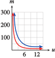
The ultraviolet index (UVI) is issued by the National Weather Service as a forecast of the amount of ultraviolet radiation expected to reach Earth around noon on a given day. The data show how much exposure to the sun people can take before risking sunburn.
| UVI | ||||||||
|---|---|---|---|---|---|---|---|---|
| Minutes to burn (more sensitive) | ||||||||
| Minutes to burn (less sensitive) |
- Plot , the minutes to burn, against , the UVI, to obtain two graphs, one for people who are more sensitive to sunburn, and another for people less sensitive to sunburn. Which of the basic functions do your graphs most resemble?
- For each graph, find a value of so that fits the data.
The shapes of the graphs resemble .- More sensitive: , Less sensitive:
To decide which basic function might model a set of data, we can
_____
To decide which basic function might model a set of data, we can plot the data.
To decide which basic function might model a set of data, we can
- plot the data.
- look at the variables.
- choose scales for the axes.
- calculate the slope.
To decide which basic function might model a set of data, we can plot the data.
At this point, a word of caution is in order. There is more to choosing a model than finding a curve that fits the data. A model based purely on the data is called an empirical model. However, many functions have similar shapes over small intervals of their input variables, and there may be several candidates that model the data. Such a model simply describes the general shape of the data set; the parameters of the model do not necessarily correspond to any actual process.
In contrast, mechanistic models provide insight into the biological, chemical, or physical process that is thought to govern the phenomenon under study. Parameters derived from mechanistic models are quantitative estimates of real system properties. Here is what GraphPad Software has to say about modeling:
"Choosing a model is a scientific decision. You should base your choice on your understanding of chemistry or physiology (or genetics, etc.). The choice should not be based solely on the shape of the graph.
"Some programs... automatically fit data to hundreds or thousands of equations and then present you with the equation(s) that fit the data best. Using such a program is appealing because it frees you from the need to choose an equation. The problem is that the program has no understanding of the scientific context of your experiment. The equations that fit the data best are unlikely to correspond to scientifically meaningful models. You will not be able to interpret the best-fit values of the variables, and the results are unlikely to be useful for data analysis."
(Source: Fitting Models to Biological Data Using Linear and Nonlinear Regression, Motulsky & Christopoulos, GraphPad Software, 2003)
Explain the difference between an empirical model and a mechanistic model.
_____
Explain the difference between an empirical model and a mechanistic model.
Modeling with Piecewise Functions
Recall that a piecewise function is defined by different formulas on different portions of the -axis.
A piecewise function
_____
none of the above
A piecewise function
- must have no breaks in its graph.
- can have more than one output at some inputs.
- cannot have concavity.
- None of the above
As part of a water conservation program, the utilities commission in Arid, New Mexico, establishes a two-tier system of monthly billing for residential water usage: The commission charges a $30 service fee plus $2 per hundred cubic feet (HCF) of water if you use 50 HCF or less, and a $50 service fee plus $3 per HCF of water if you use over 50 HCF (1 HCF of water is about 750 gallons).
- Write a piecewise formula for the water bill, , as a function of the amount of water used, , in HCF.
where _____
and _____ - Graph the function .
- A graph is below.
A graph for part (b):
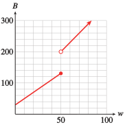
As part of a water conservation program, the utilities commission in Arid, New Mexico, establishes a two-tier system of monthly billing for residential water usage. The commission charges a $30 service fee plus $2 per hundred cubic feet (HCF) of water if you use 50 HCF or less, and a $50 service fee plus $3 per HCF of water if you use over 50 HCF. (1 HCF of water is about 750 gallons).
- Write a piecewise formula for the water bill, , as a function of the amount of water used, , in HCF.
- Graph the function .
Explain how slope and concavity are related.
_____
Explain how slope and concavity are related.
Section Summary
Vocabulary
Look up the definitions of new terms in the Glossary.
- Increasing
- Decreasing
- Concave up
- Concave down
- Empirical model
- Mechanistic model
CONCEPTS
- The shape of a graph describes how the output variable changes.
- A nonlinear graph may be concave up or concave down. If a graph is concave up, its slope is increasing. If it is concave down, its slope is decreasing.
- The basic functions can be used to model physical situations.
- Some situations can be modeled by piecewise functions
- Fitting a curve to the data is not enough to produce a useful model; appropriate scientific principles should also be considered.
STUDY QUESTIONS
- Sketch the graph of a function whose slope is positive and increasing.
- Sketch the graph of a function whose slope is positive and decreasing.
- Which basic function is increasing but bending downward?
- Which basic function is decreasing but bending upward?
- Why is it bad practice to choose a model purely on the shape of the data plot?
SKILLS
Practice each skill in the Homework problems listed.
- Sketch a graph whose shape models a situation: #1–18
- Choose one of the basic graphs to fit a situation or a set of data: #19–24, 35–44
- Decide whether the graph of a function is increasing or decreasing, concave up or concave down from a table of values: #25–28
- Write and sketch a piecewise define function to model a situation: #45–48
Homework 2.4
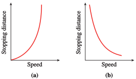
In Problems 1–4, which graph best illustrates each of the following situations?
Your pulse rate during an aerobics class
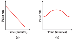
(b)
The stopping distances for cars traveling at various speeds
Your income in terms of the number of hours you worked
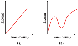
(a)
Your temperature during an illness
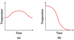
In Problems 5–8, sketch graphs to illustrate the following situations
Halfway from your English class to your math class, you realize that you left your math book in the classroom. You retrieve the book, then walk to your math class. Graph the distance between you and your English classroom as a function of time, from the moment you originally leave the English classroom until you reach the math classroom.
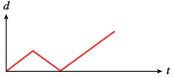
After you leave your math class, you start off toward your music class. Halfway there you meet an old friend, so you stop and chat for a while. Then you continue to the music class. Graph the distance between you and your math classroom as a function of time, from the moment you leave the math classroom until you reach the music classroom.
Toni drives from home to meet her friend at the gym, which is halfway between their homes. They work out together at the gym; then they both go to the friend's home for a snack. Finally Toni drives home. Graph the distance between Toni and her home as a function of time, from the moment she leaves home until she returns.
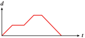
While bicycling from home to school, Greg gets a flat tire. He repairs the tire in just a few minutes but decides to backtrack a few miles to a service station, where he cleans up. Finally, he bicycles the rest of the way to school. Graph the distance between Greg and his home as a function of time, from the moment he leaves home until he arrives at school.
Choose the graph that depicts the function described in Problems 9 and 10.
Inflation is still rising, but by less each month.
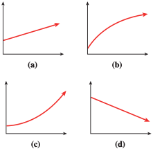
(b)
The price of wheat was rising more rapidly in 1996 than at any time during the previous decade.
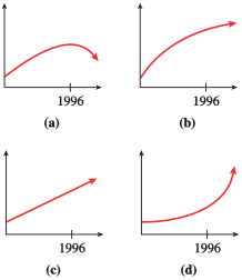
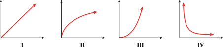
In Problems 11 and 12, match each graph with the function it illustrates.
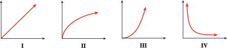
- The volume of a cylindrical container of constant height as a function of its radius
- The time it takes to travel a fixed distance as a function of average speed
- The simple interest earned at a given interest rate as a function of the investment
- The number of Senators present versus the number absent in the U.S. Senate
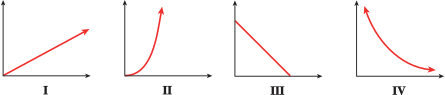
- II
- IV
- I
- III
- Unemployment was falling but is now steady.
- Inflation, which rose slowly until last month, is now rising rapidly.
- The birthrate rose steadily until 1990 but is now beginning to fall.
- The price of gasoline has fallen steadily over the past few months.
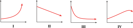
Sketch possible graphs to illustrate the situations described in Problems 13–18.
The height of a man as a function of his age, from birth to adulthood
The number of people willing to buy a new high-definition television, as a function of its price
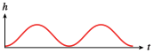
The height of your head above the ground during a ride on a Ferris wheel
The height above the ground of a rubber ball dropped from the top of a -foot ladder
The average age at which women first marry decreased from 1940 to 1960, but it has been increasing since then
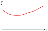
When you learn a foreign language, the number of vocabulary words you know increases slowly at first, then increases more rapidly, and finally starts to level off.
Each situation in Problems 19–24 can be modeled by a transformation of a basic function. Name the basic function and sketch a possible graph.
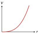
The volume of a hot air balloon, as a function of its radius
stretched or compressed vertically
The length of a rectangle as a function of its width, if its area is square feet
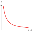
The time it takes you to travel miles, as a function of your average speed
stretched or compressed vertically
The sales tax on a purchase, as a function of its price
The width of a square skylight, as a function of its area
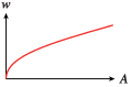
The area of a circle as a function of its diameter
In Problems 25–28, use the table of values to answer the questions.
- Based on the given values, is the function increasing or decreasing?
- Could the function be concave up, concave down, or linear?
- Increasing
- Concave up
- Increasing
- Concave down
In Problems 29–34,
- Is the graph increasing or decreasing, concave up or concave down?
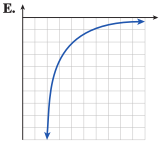
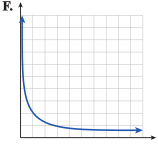
- Match the graph of the function with the graph of its rate of change, shown in Figures A–F.
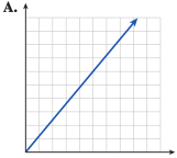
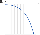
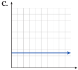
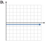
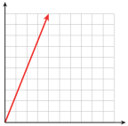
- Increasing, linear (neither concave up nor down)
- C
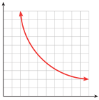
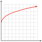
- Increasing, concave down
- F
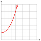
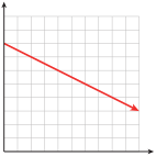
- Decreasing, linear (neither concave up nor down)
- D
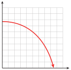
For Problems 35–40, plot the data; then decide which of the basic functions could describe the data.
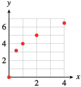
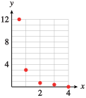
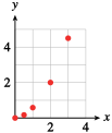
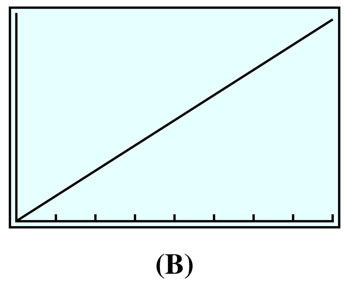
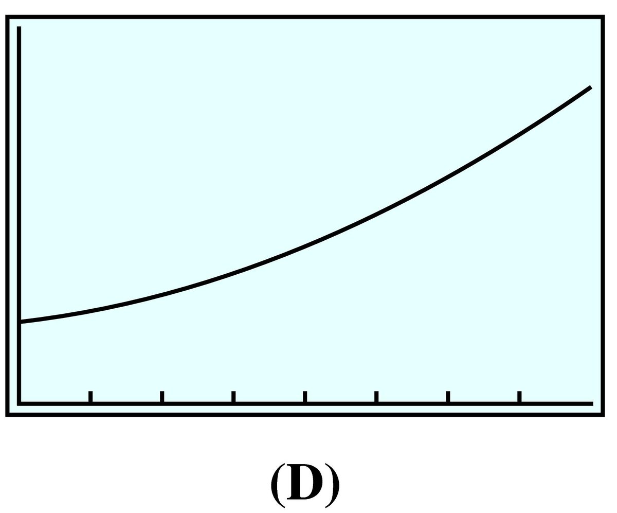
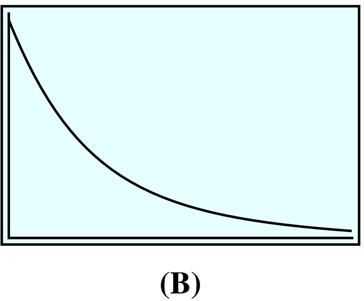
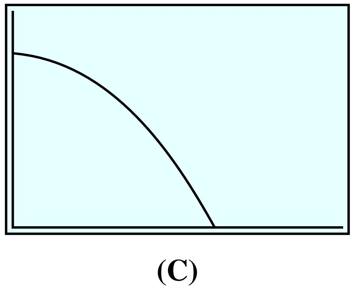
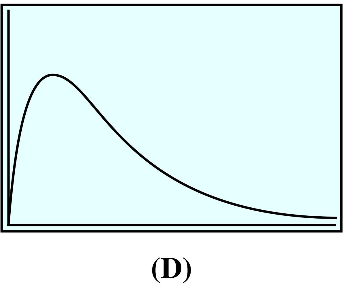
Four different functions are described below. Match each description with the appropriate table of values and with its graph.
- As a chemical pollutant pours into a lake, its concentration is a function of time. The concentration of the pollutant initially increases quite rapidly, but due to the natural mixing and self-cleansing action of the lake, the concentration levels off and stabilizes at some saturation level.
- An overnight express train travels at a constant speed across the Great Plains. The train's distance from its point of origin is a function of time.
- The population of a small suburb of a Florida city is a function of time. The population began increasing rather slowly, but it has continued to grow at a faster and faster rate.
- The level of production at a manufacturing plant is a function of capital outlay, that is, the amount of money invested in the plant. At first, small increases in capital outlay result in large increases in production, but eventually the investors begin to experience diminishing returns on their money, so that although production continues to increase, it is at a disappointingly slow rate.
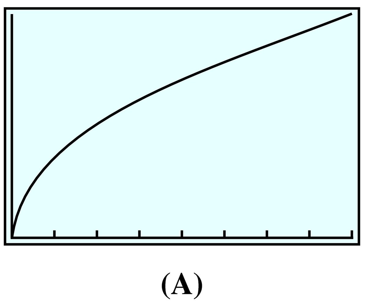
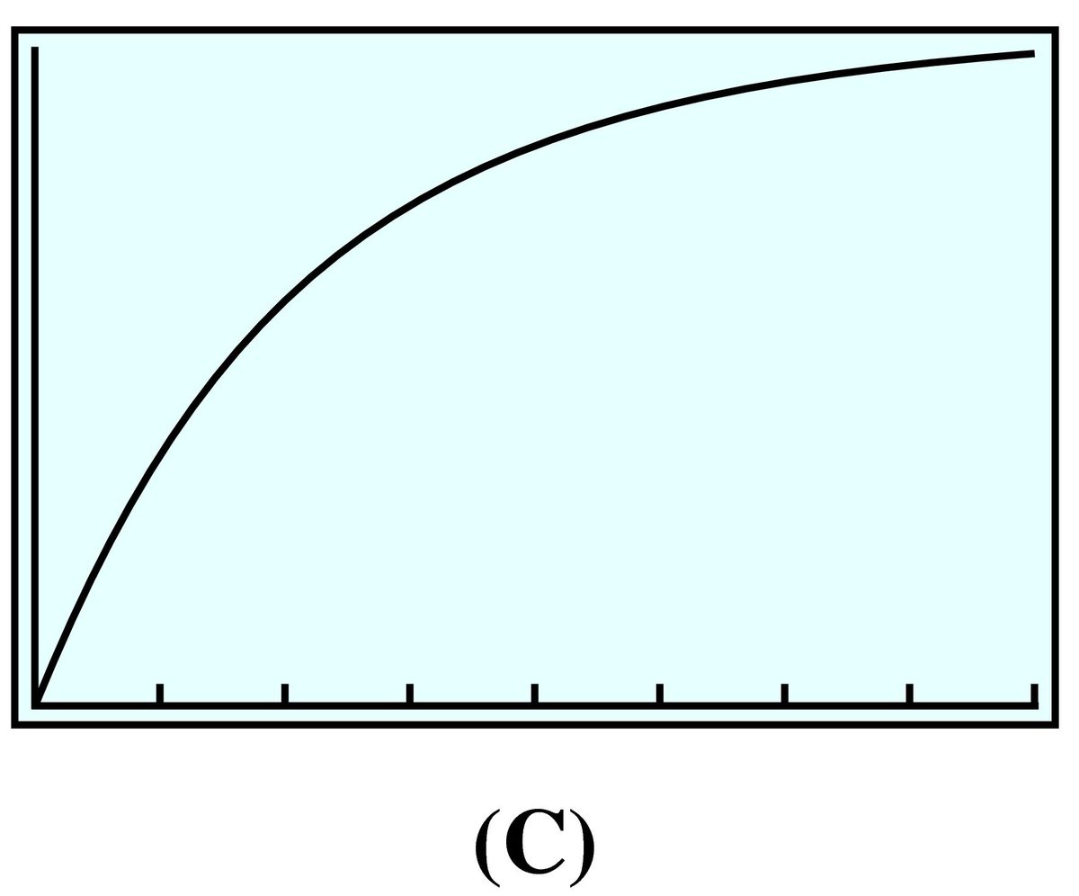
- Table (4), Graph (C)
- Table (3), Graph (B)
- Table (1), Graph (D)
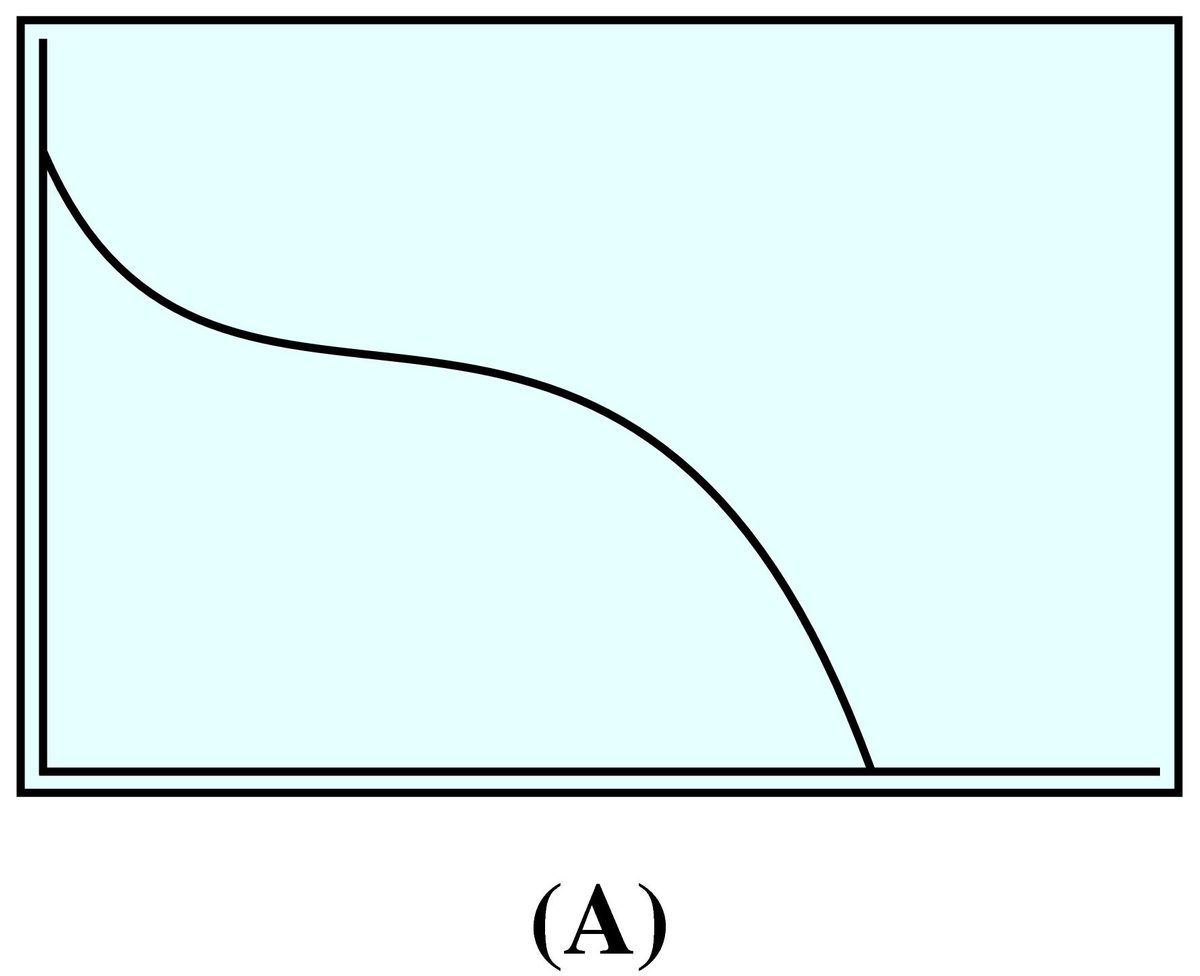
- Table (2), Graph (A)
Four different functions are described below. Match each description with the appropriate table of values and with its graph.
- Fresh water flowing through Crystal Lake has gradually reduced the phosphate concentration to its natural level, and it is now stable.
- The number of bacteria in a person during the course of an illness is a function of time. It increases rapidly at first, then decreases slowly as the patient recovers.
- A squirrel drops a pine cone from the top of a California redwood. The height of the pine cone is a function of time, decreasing ever more rapidly as gravity accelerates its descent.
- Enrollment in Ginny's Weight Reduction program is a function of time. It began declining last fall. After the holidays, enrollment stabilized for a while but soon began to fall off again.
The table shows the radii, , of several gold coins, in centimeters, and their value, , in dollars.
| Radius | |||||
|---|---|---|---|---|---|
| Value |
- Which graph represents the data?
- Which equation describes the function?
- III
- 3
The table shows how the amount of water, , flowing past a point on a river is related to the width, , of the river at that point.
| Width (feet) | ||||
|---|---|---|---|---|
| Amount of water |
- Which graph represents the data?
- Which equation describes the function?
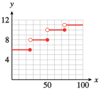
If you order from Coldwater Creek, the shipping charges are given by the following table.
| Purchase amount | Shipping charge |
|---|---|
| Up to $25 | $5.95 |
| $25.01 to $50 | $7.95 |
| $50.01 to $75 | $9.95 |
| $75.01 to $100 | $10.95 |
- Write a piecewise formula for , the shipping charge as a function of the purchase amount, .
- Graph .
The Bopp-Busch Tool and Die Company markets its products to individuals, to contractors, and to wholesale distributors. The company offers three different price structures for its toggle bolts. If you order or fewer boxes, the price is $ each. If you order more than but no more than boxes, the price is $ each. If you order more than boxes, the price is $ each.
- Write a piecewise formula for , the cost of ordering boxes of toggle bolts.
- Graph .
Bob goes skydiving on his birthday. The function approximates Bob's altitude seconds into the trip.
- Graph . Describe what you think is happening during each piece of the graph.
- Find two times when Bob is at an altitude of feet.
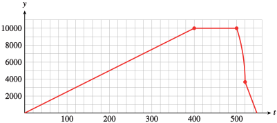
During the first 400 seconds Bob's altitude is climbing with the aircraft; then the aircraft maintains a constant altitude of 10,000 feet for the next 100 seconds; after jumping from the plane, Bob falls for 20 seconds before opening the parachute; he falls at a constant rate after the chute opens.- seconds (4 minutes) and
Jenni lives in the San Fernando Valley, where it is hot during summer days but cools down at night. Jenni uses the air conditioner as little as possible. The function approximates the temperature in Jenni's house hours after midnight.
- Graph . Describe what you think is happening during each piece of the graph.
- Find two times when the temperature inside the house is Fahrenheit.
Lead nitrate and potassium iodide react in solution to produce lead iodide, which settles out, or precipitates, as a yellow solid at the bottom of the container. As you add more lead nitrate to the solution, more lead iodide is produced until all the potassium iodide is used up. The table shows the height of the precipitate in the container as a function of the amount of lead nitrate added. (Source: Hunt and Sykes, 1984)
| Lead nitrate solution (cc) | ||||||||
|---|---|---|---|---|---|---|---|---|
| Height of precipitate (mm) |
- Plot the data. Sketch a piecewise linear function with two parts to fit the data points
- Calculate the slope of the increasing part of the graph, including units. What is the significance of the slope?
- Write a formula for your piecewise function.
- Interpret your graph in the context of the problem.
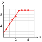
- mm/cc: The height of precipitate increases by mm for each additional cc of lead nitrate
- The increasing portion of the graph corresponds to the period when the reaction was occurring, and the horizontal section corresponds to when the potassium iodide is used up.
The graph shows the temperature of gram of water as a function of the amount of heat applied, in calories. Recall that water freezes at C and boils at C.
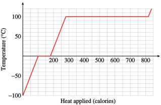
- How much heat is required to raise the temperature of gram of water by degree?
- How much heat is required to convert gram of ice to water?
- How much heat is required to convert gram of water to steam?
- Write a piecewise function to describe the graph.
As the global population increases, many scientists believe it is approaching, or has already exceeded, the maximum number the Earth can sustain. This maximum number, or carrying capacity, depends on the finite natural resources of the planet—water, land, air, and materials—but also on how people use and preserve the resources. The graphs show four different ways that a growing population can approach its carrying capacity over time. (Source: Meadows, Randers, and Meadows, 2004)
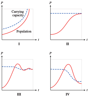
Match each graph to one of the scenarios described in (a)–(d) and explain your choice.
- Sigmoid growth: The population levels off smoothly below the carrying capacity.
- Overshoot and collapse: The population exceeds the carrying capacity with severe damage to the resource base and is forced to decline rapidly to achieve a new balance with a reduced carrying capacity.
- Continued growth: The carrying capacity is far away, or growing faster than the population.
- Overshoot and oscillation: The population exceeds the carrying capacity without inflicting permanent damage, then oscillates around the limit before leveling off.
- II
- IV
- I
- III
The introduction of a new species into an environment can affect the growth of an existing species in various ways. The graphs show four hypothetical scenarios after Species A is introduced into an environment where Species B is established.
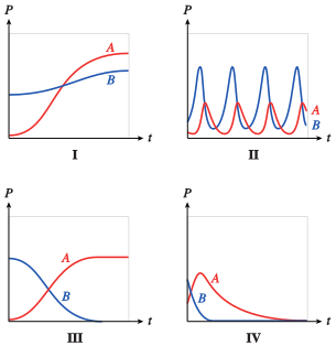
Match each graph to one of the scenarios described in (a)–(d) and explain your choice.
- Predator-prey (sustained): Species A becomes a predator population that grows when its prey, Species B, is abundant, but declines when the prey population is small. The prey population grows when predators are scarce but shrinks when predators are abundant.
- Predator-prey (extinction): Species A becomes a predator population that annihilates Species B, but then Species A itself declines toward extinction.
- Competition: Species A and B have a common food source, and the Species A replaces Species B in the environment.
- Symbiosis: Species A and B help each other to grow.
Modeling, Functions, and Graphs by Katherine Yoshiwara (yoshiwarabooks.org), GNU Free Documentation License 1.2 or later. Adapted for the XYZ HTML edition with the authors' permission (recorded 2026-07-04). License: GFDL-1.2-or-later.