
7.2 Graphing Polynomial Functions
In Polynomial Functions, we considered applications of polynomial functions. Although most applications use only a portion of the graph of a particular polynomial, we can learn a lot about these functions by taking a more global view of their behavior.
Classifying Polynomials by Degree
The graph of a polynomial function depends first of all on its degree. We have already studied the graphs of polynomials of degrees , , and .
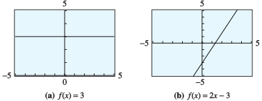
- A polynomial of degree is a constant, and its graph is a horizontal line. An example of such a polynomial function is .
- A polynomial of degree is a linear function, and its graph is a straight line. The function is an example of a polynomial of degree .
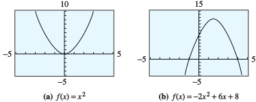
- Quadratic functions, such as , are polynomials of degree . The graph of every quadratic function is a parabola, with the same basic shape as the standard parabola, . It has one turning point, where the graph changes from increasing to decreasing or vice versa. The turning point of a parabola is the same as its vertex.
Cubic Polynomials
Do the graphs of all cubic, or third-degree, polynomials have a basic shape in common? We can graph a few examples and find out. Unlike the basic parabola, the graph of is always increasing. At the origin, however, it changes from concave down to concave up. A point where the graph changes concavity is called an inflection point.
At an inflection point, a graph changes
_____
A graph changes concavity at an inflection point.
At an inflection point, a graph changes
- direction.
- concavity.
- sign.
- all of these.
Despite the differences in the central portions of the two graphs, they exhibit similar long-term behavior.
- For very large and very small values of , both graphs look like the power function .
- The -values increase from toward zero in the third quadrant, and they increase from zero toward in the first quadrant. Or we might say that the graphs start at the lower left and extend to the upper right.
All cubic polynomials display this behavior when their lead coefficients (the coefficient of the term) are positive.
- Both of the graphs in Example are smooth curves without any breaks or holes. This smoothness is a feature of the graphs of all polynomial functions.
- The domain of any polynomial function is the entire set of real numbers.
- Complete the table of values below for .
_____ _____ _____ _____ _____ _____ _____ _____ _____ - Graph in the standard window. Compare the graph to the graphs in the Example above: What similarities do you notice? What differences?
- Both non-basic cubic graphs have three -intercepts and two turning points. _____
- Both non-basic cubic graphs have the same long-term behavior as . _____
- The non-basic cubic function from the example has three -intercepts and two turning points, but this cubic function has only one turning point. _____
- The non-basic cubic function from the example has long-term behavior like , but his cubic function has long-term behavior like . _____
- A graph is below.
Both graphs have three -intercepts, but the function in the Example above has long-term behavior like , and this function has long-term behavior like .
A graph for part (b):
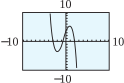
- Complete the table of values below for .
- Graph in the standard window. Compare the graph to the graphs in the Example above: What similarities do you notice? What differences?
Both graphs have three -intercepts, but the function in the Example above has long-term behavior like , and this function has long-term behavior like .
Quartic Polynomials
Now let’s compare the long-term behavior of two quartic, or fourth-degree, polynomials.
- Complete the following table of values for .
_____ _____ _____ _____ _____ _____ _____ _____ _____ - Graph in the window
Compare the graph to the graphs in the previous Example: What similarities do you notice? What differences?
- The graphs all have four -intercepts and three turning points. _____
- The graphs all have long-term behavior like a fourth degree power function, . _____
- The long-term behavior of the graphs in the example is the same as that of , but the graph here has long-term behavior like . _____
- The long-term behavior of the graphs in the example is the same as that of , but the graph here has long-term behavior like . _____
- The graphs all have long-term behavior like a fourth degree power function, . The long-term behavior of the graphs in the Example is the same as that of , but the graph here has long-term behavior like .
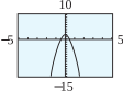
A graph for part (b):
- Complete the following table of values for .
- Graph in the window Compare the graph to the graphs in the previous Example: What similarities do you notice? What differences?
The graphs all have long-term behavior like a fourth degree power function, . The long-term behavior of the graphs in the Example is the same as that of , but the graph here has long-term behavior like .
In Examples and Example, we have seen polynomials of degree 3 and degree 4, whose graphs are illustrated in the next box. In the Homework Problems, you will consider more graphs to help you verify the following observations.
The long-term behavior of a polynomial of degree
_____
is the same as the behavior of .
The long-term behavior of a polynomial of degree
- depends on the number of its zeros.
- is the same as the behavior of .
- may have a horizontal asymptote.
- cannot be determined without a graph.
-Intercepts and the Factor Theorem
In Quadratic Functions, we saw that the x-intercepts of a quadratic polynomial, , occur at values of for which , that is, at the real-valued solutions of the equation . The same holds true for polynomials of higher degree.
Solutions of the equation are called zeros of the polynomial . In Example, we graphed the cubic polynomial . Its -intercepts are the solutions of the equation , which we can solve by factoring the polynomial .
The zeros of are , , and . Each zero of corresponds to a factor of . This result suggests the following theorem, which holds for any polynomial .
Without graphing, how can you tell that the polynomial has no -intercepts?
_____
It cannot be factored further. Because the two quadratic factors are both positive for all , their product is always positive.
Without graphing, how can you tell that the polynomial has no -intercepts?
- It is quartic.
- All of its coefficients are positive.
- It cannot be factored further.
- It has no turning points.
The factor theorem follows from the division algorithm for polynomials. (See the Polynomials and Factoring section in Appendix Algebra Skills Refresher to review polynomial division.) We will consider both of these results in more detail in the Homework problems.
The graph of which type of polynomial must have an -intercept?
_____
The graph of any cubic polynomial must have at least one -intercept.
The graph of which type of polynomial must have an -intercept?
- Quadratic
- Cubic
- Quartic
- None of these
Because a polynomial function of degree can have at most linear factors of the form , it follows that can have at most distinct zeros.
Another way of saying this is that if is a polynomial of th degree, the equation can have at most distinct solutions, some of which may be complex numbers. (We consider complex numbers in Complex Numbers.)
Because only real-valued solutions appear on the graph as -intercepts, we have the following corollary to the factor theorem.
If some of the zeros of are complex numbers, they will not appear on the graph, so a polynomial of degree may have fewer than -intercepts.
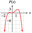
- Find the real-valued zeros of by factoring.
_____ Separate different zeros with a comma. - Sketch a rough graph of by hand.
- A graph is below.
Graph for part (b):
- Find the real-valued zeros of by factoring.
- Sketch a rough graph of by hand.
How may the graph of a polynomial differ from the graph of a power function of the same degree?
_____
How may the graph of a polynomial differ from the graph of a power function of the same degree?
Zeros of Multiplicity Two or Three
The appearance of the graph near an -intercept is determined by the multiplicity of the zero there.
- Both real zeros of the polynomial in Exampleb are of multiplicity one, and the graph crosses the -axis at each intercept.
- The polynomial in Examplea has a zero of multiplicity two at . The graph of just touches the -axis and then reverses direction without crossing the axis.
To understand what happens in general, compare the graphs of the three polynomials below.
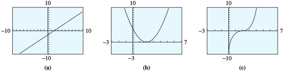
- In figure (a), has a zero of multiplicity one at , and its graph crosses the -axis there.
- In figure (b), has a zero of multiplicity two at , and its graph touches the -axis there but changes direction without crossing.
- In figure (c), has a zero of multiplicity three at . In this case, the graph makes an S-shaped curve at the intercept, like the graph of .
Near its -intercepts, the graph of a polynomial takes one of the characteristic shapes illustrated above.
Sketch a rough graph of by hand. Label the - and -intercepts.
has degree three with a positive coefficient of , so its graph starts at the lower left and extends to the upper right. The graph crosses the -axis at , touches the -axis at the double zero and then changes direction, as shown in the graph below.
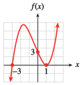
Sketch a rough graph of by hand. Label the - and -intercepts.
has degree three with a positive coefficient of , so its graph starts at the lower left and extends to the upper right. The graph crosses the -axis at , touches the -axis at the double zero and then changes direction, as shown in the graph below.
Explain how the multiplicity of a zero affects the shape of the graph near that zero.
_____
Explain how the multiplicity of a zero affects the shape of the graph near that zero.
Section Summary
Vocabulary
Look up the definitions of new terms in the Glossary.
- Degree
- Multiplicity
- Inflection point
- Quartic
- Turning point
- Cubic
- Corollary
- Zero
CONCEPTS
- The graphs of all polynomials are smooth curves without breaks or holes.
- The graph of a polynomial of degree (with positive leading coefficient) has the same long-term behavior as the power function of the same degree.
- A polynomial of degree can have at most -intercepts.
- At a zero of multiplicity two, the graph of a polynomial has a turning point. At a zero of multiplicity three, the graph of a polynomial has an inflection point.
STUDY QUESTIONS
- Describe the graphs of polynomials of degrees , , and .
- What does the degree of a polynomial tell you about its long-term behavior?
- What is a zero of a polynomial?
- How are zeros related to the factors of a polynomial?
- What do the zeros tell you about the graph of a polynomial?
- Explain the difference between a turning point and an inflection point.
SKILLS
Practice each skill in the Homework problems listed.
- Identify -intercepts, turning points, and inflection points: #1–8, 11–18
- Use a graph to factor a polynomial: #21–28
- Sketch the graph of a polynomial: #29–46
- Find a possible formula for a polynomial whose graph is shown: #47–52
- Graph translations of polynomials: #53–56
Homework 7.2
In Problems 1–8, use your calculator to graph each cubic polynomial.
- Describe the long-term behavior of each graph. How does this behavior compare to that of the basic cubic? How does the sign of the lead coefficient affect the graph?
- How many -intercepts does each graph have? How many turning points? How many inflection points?
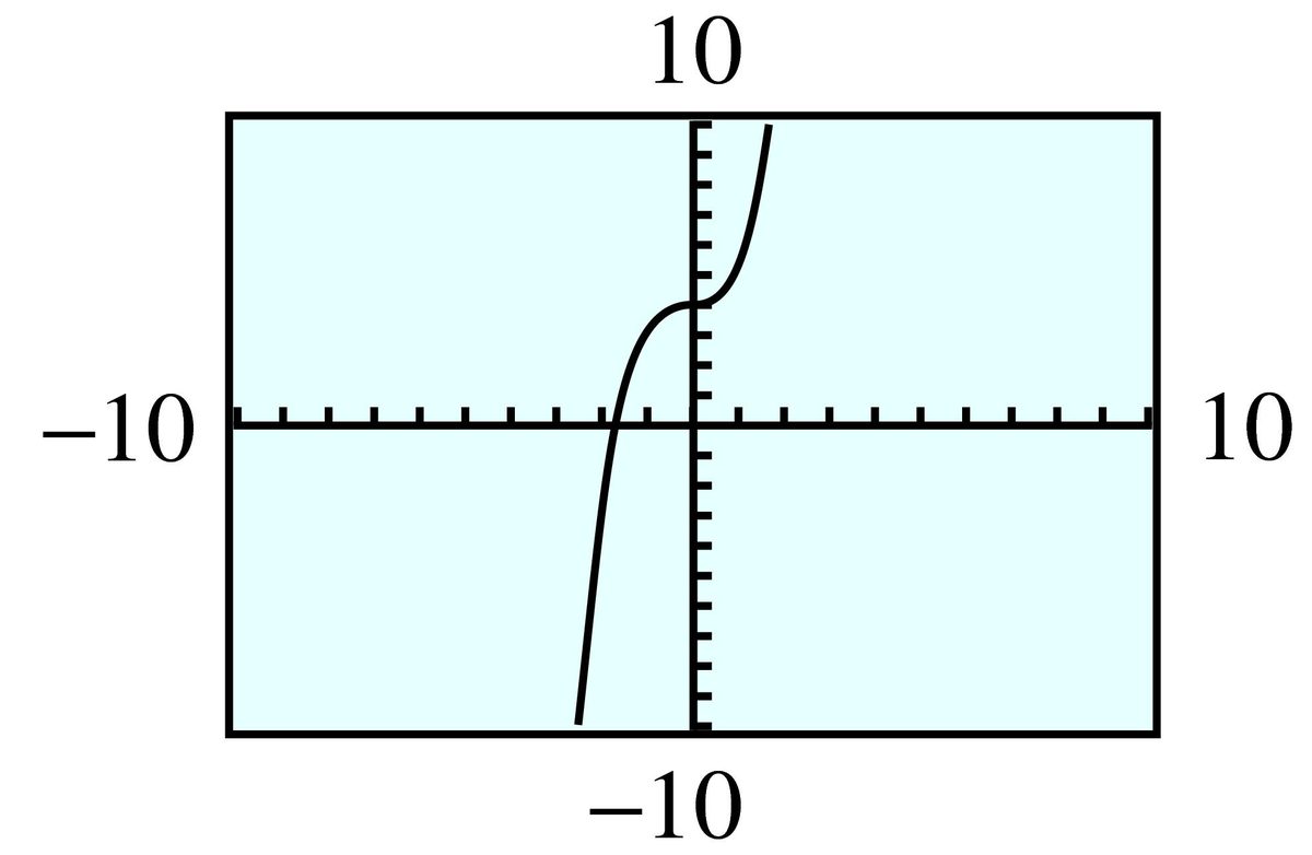
- The end behavior is the same as for the basic cubic because the lead coefficient is positive.
- There is one -intercept, no turning points, one inflection point.
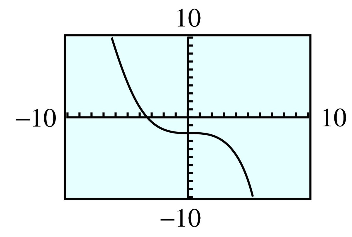
- The end behavior is the opposite to the basic cubic (the graph starts in the upper left and extends to the lower right) because the lead coefficient is negative.
- There is one -intercept, no turning points, one inflection point.
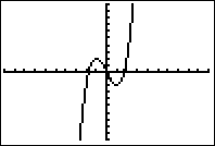
- The end behavior is the same as for the basic cubic because the lead coefficient is positive.
- There are three -intercepts, two turning points, one inflection point.
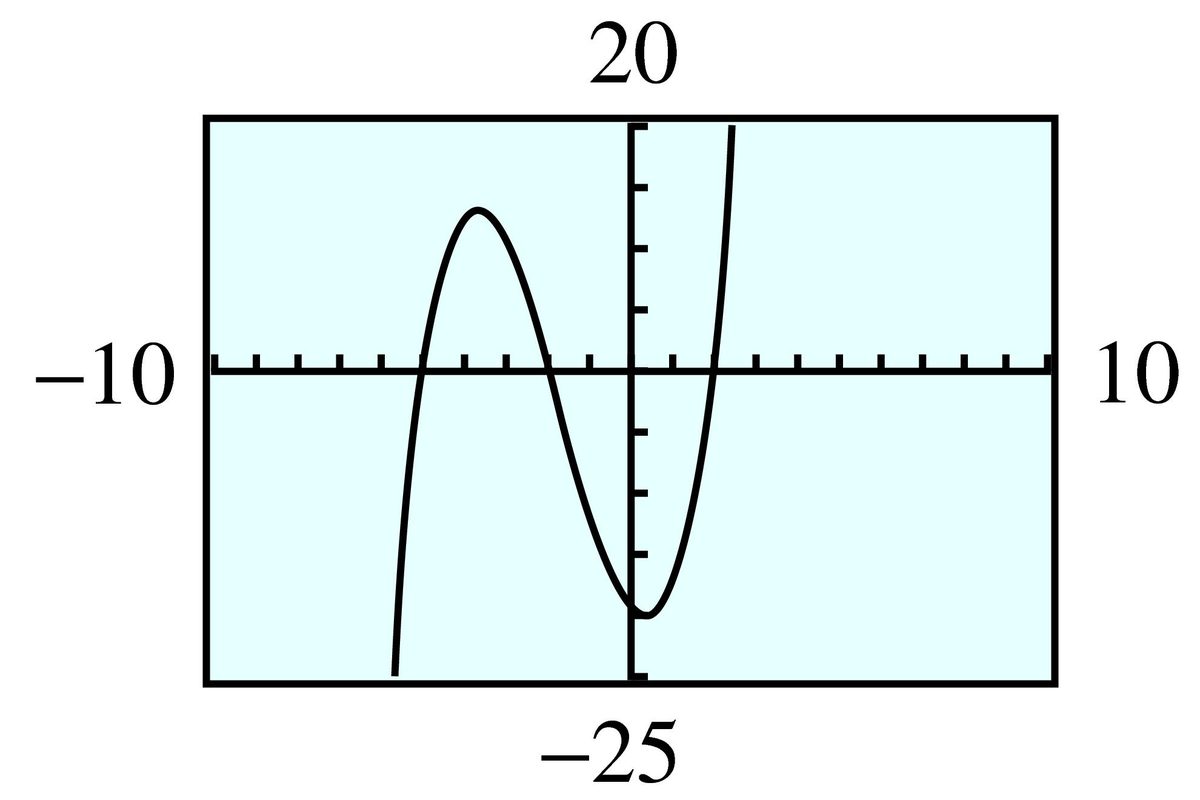
- The end behavior is the same as for the basic cubic because the lead coefficient is positive.
- There are three -intercepts, two turning points, one inflection point.
For Problems 9–10, use a graphing utility to graph each cubic polynomial. Which graphs are the same?
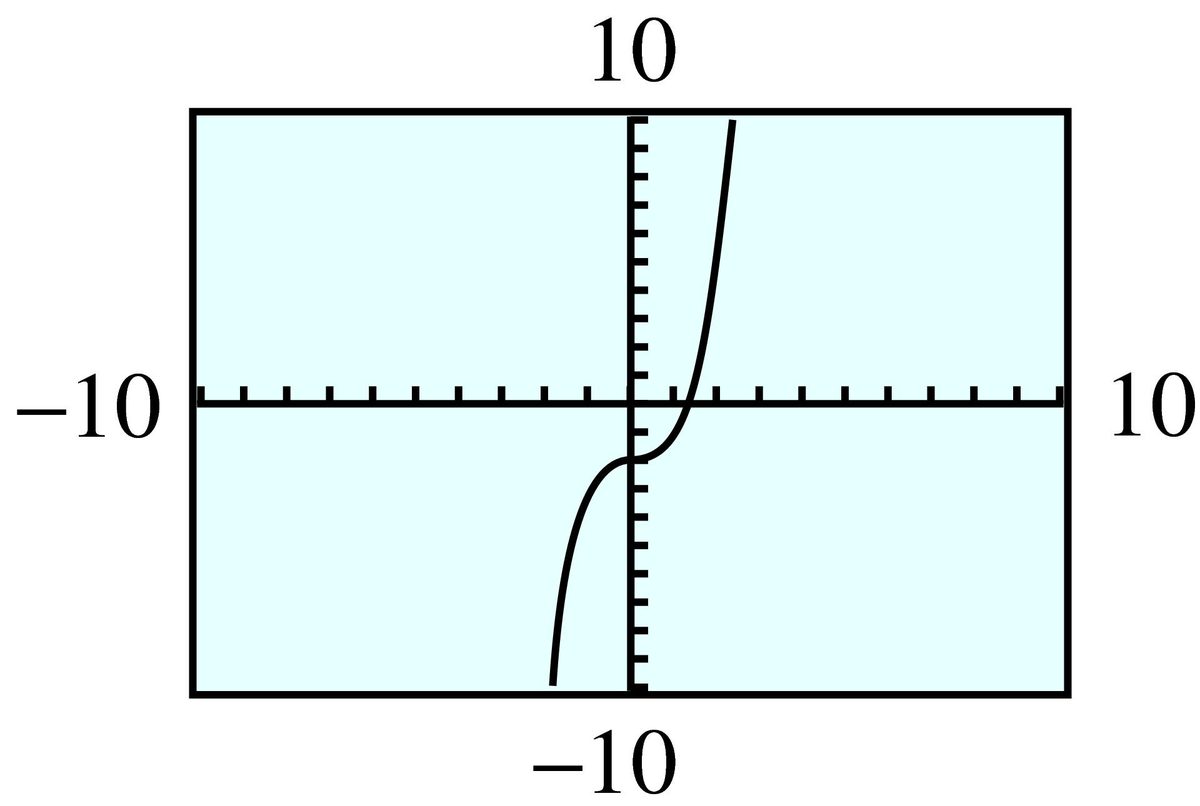
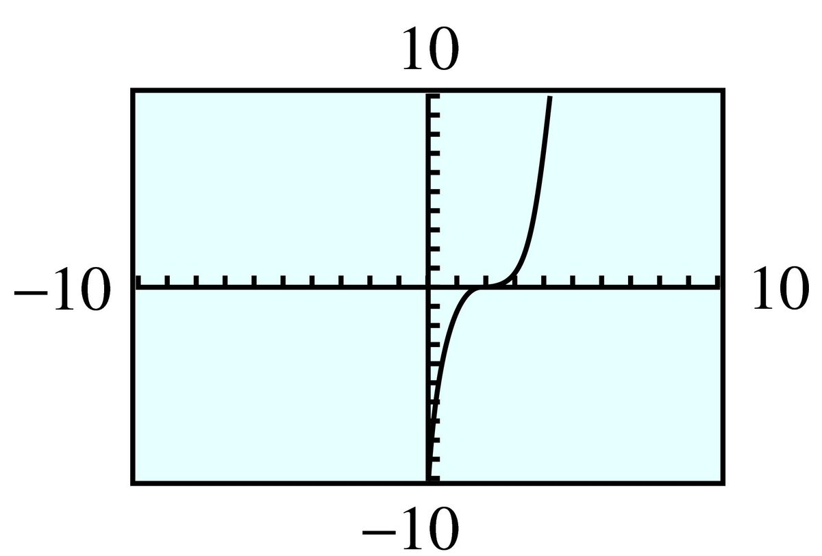
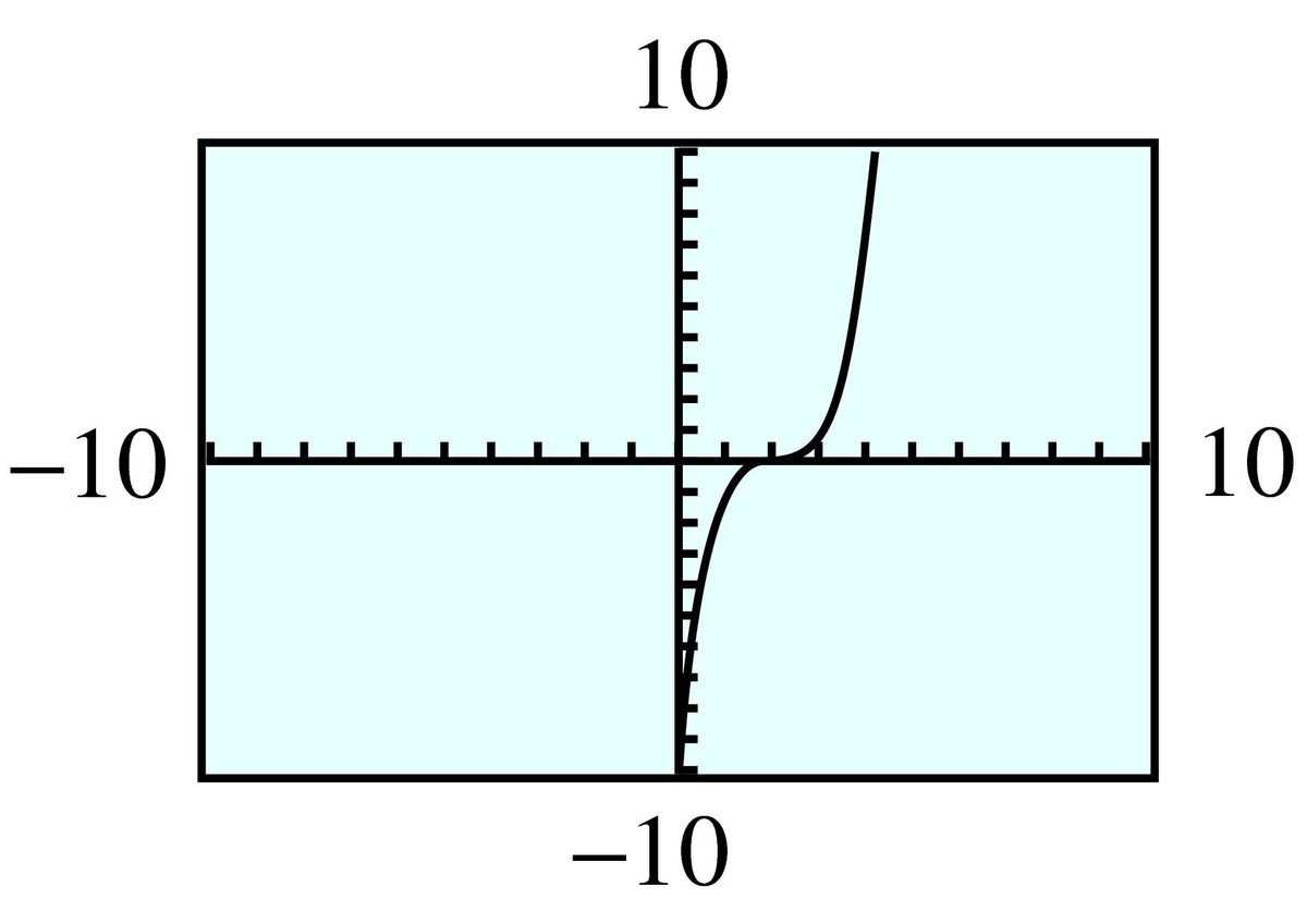
(b) and (c) are the same.
In Problems 11–18, use your calculator to graph each quartic polynomial.
- Describe the long-term behavior of each graph. How does this behavior compare to that of the basic quartic? How does the sign of the lead coefficient affect the graph?
- How many -intercepts does each graph have? How many turning points? How many inflection points?
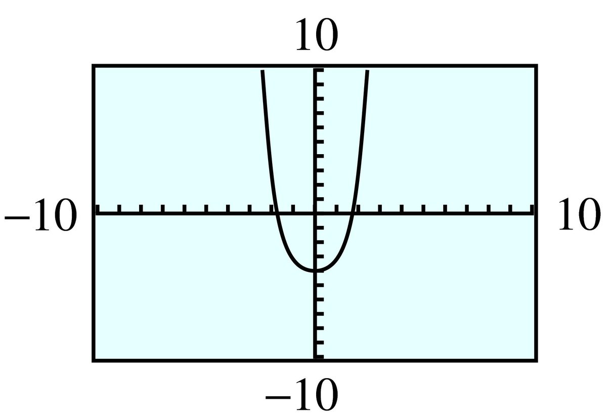
- The end behavior is the same as for the basic quartic because the lead coefficient is positive.
- There are two -intercepts, one turning point, no inflection point.
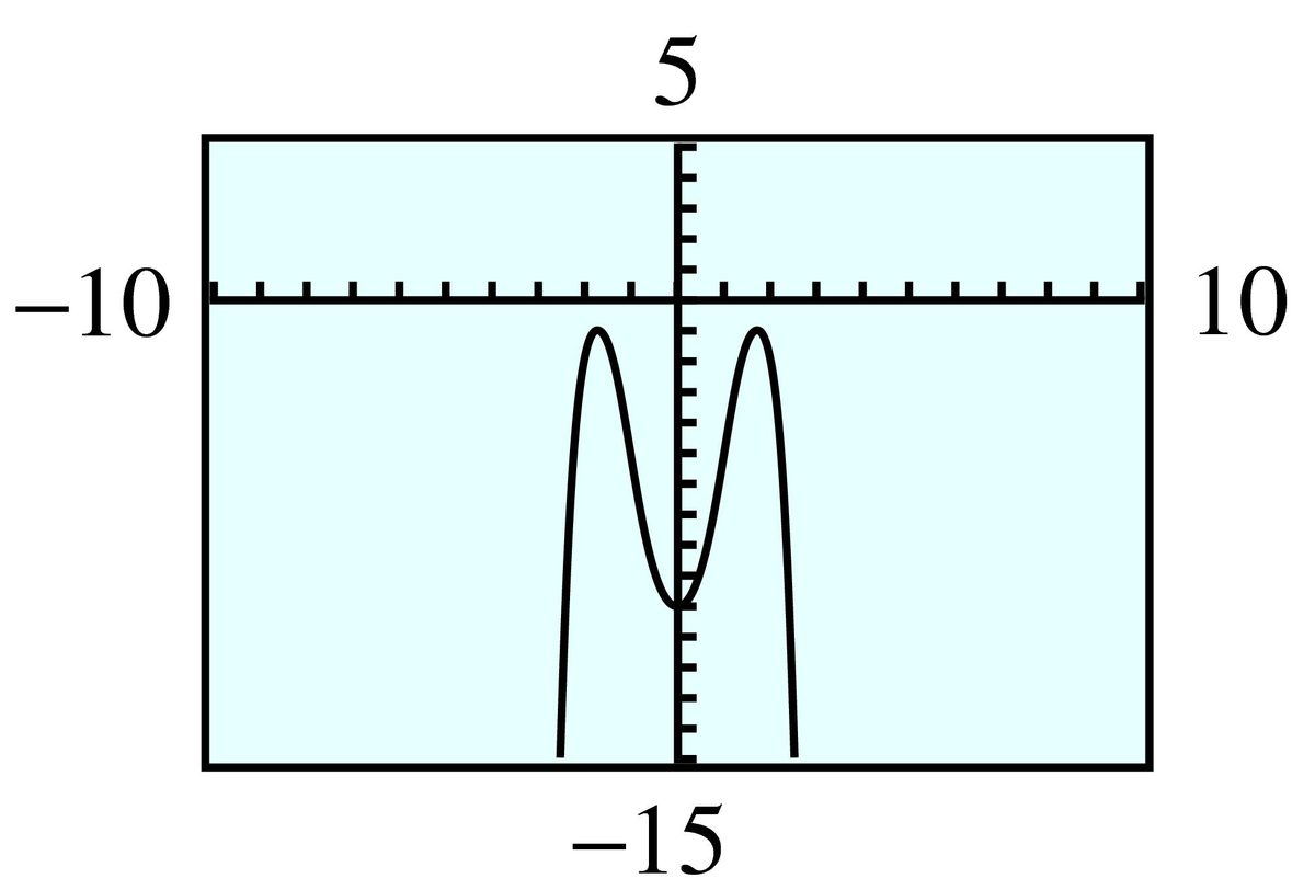
- The end behavior is the opposite of the basic quartic (the graph starts in the lower left and ends in the lower right) because the lead coefficient is negative.
- There are no -intercepts, three turning points, two inflection points.
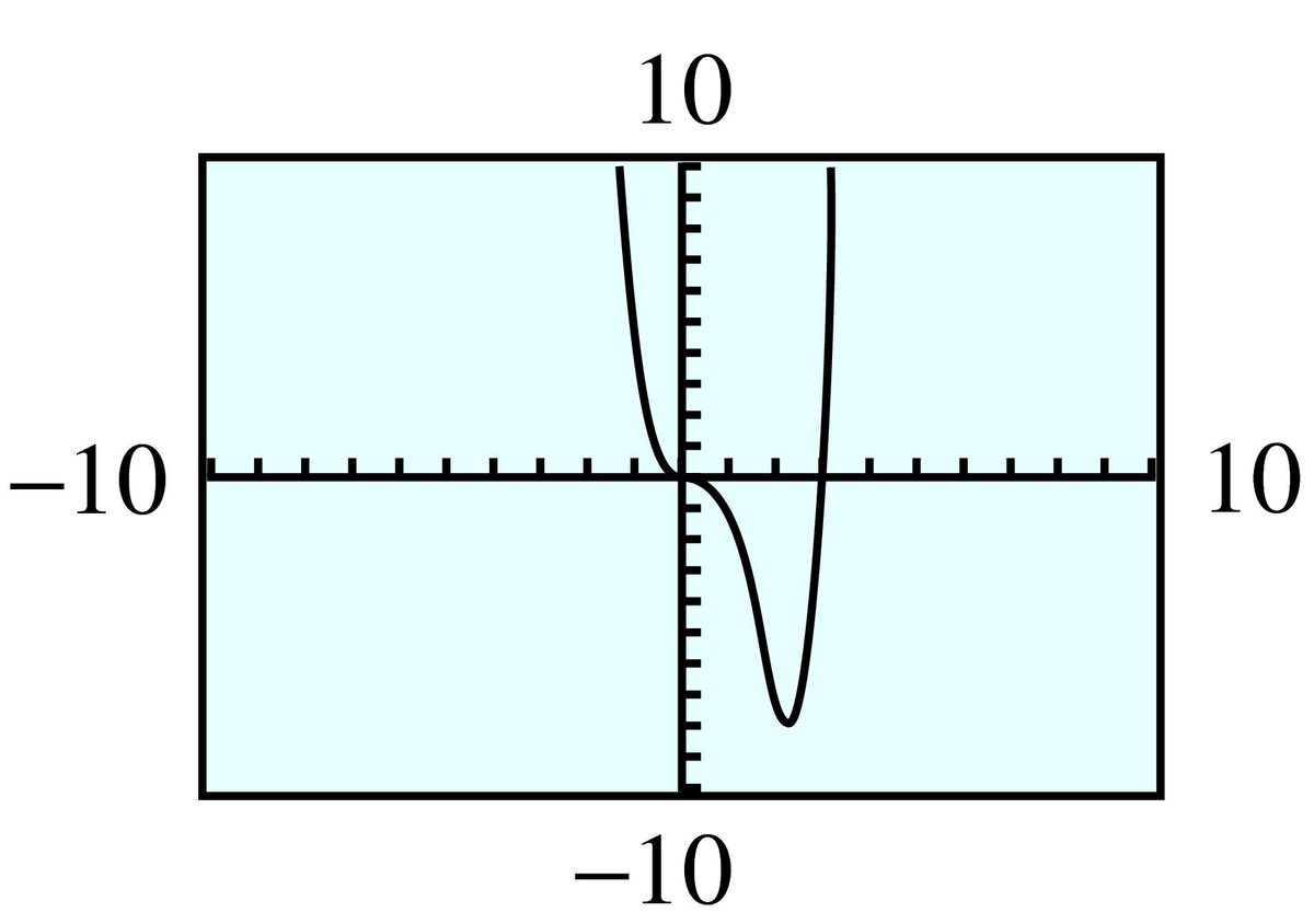
- The end behavior is the same as for the basic quartic because the lead coefficient is positive.
- There are two -intercepts, one turning point, two inflection points.
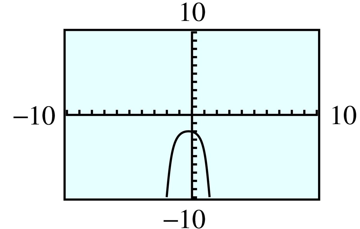
- The end behavior is the opposite of the basic quartic (the graph starts in the lower left and ends in the lower right) because the lead coefficient is negative.
- There are no -intercepts, one turning point, two inflection points.
From your answers to Problems 1–8, what you can conclude about the graphs of cubic polynomials? Consider the long-term behavior, -intercepts, turning points, and inflection points.
The graph of a cubic polynomial with a positive lead coefficient will have the same end behavior as the basic cubic, and a cubic with a negative lead coefficient will have the opposite end behavior. Each graph of a cubic polynomial has one, two, or three -intercepts, it has two, one or no turning point, and it has exactly one inflection point.
From your answers to Problems 11–18, what you can conclude about the graphs of quartic polynomials? Consider the long-term behavior, -intercepts, turning points, and inflection points.
For Problems 21–28,
- Use your calculator to graph each polynomial and locate the -intercepts. Set , , and adjust and to get a good graph.
- Write the polynomial in factored form.
- Expand the factored form of the polynomial (that is, multiply the factors together). Do you get the original polynomial?
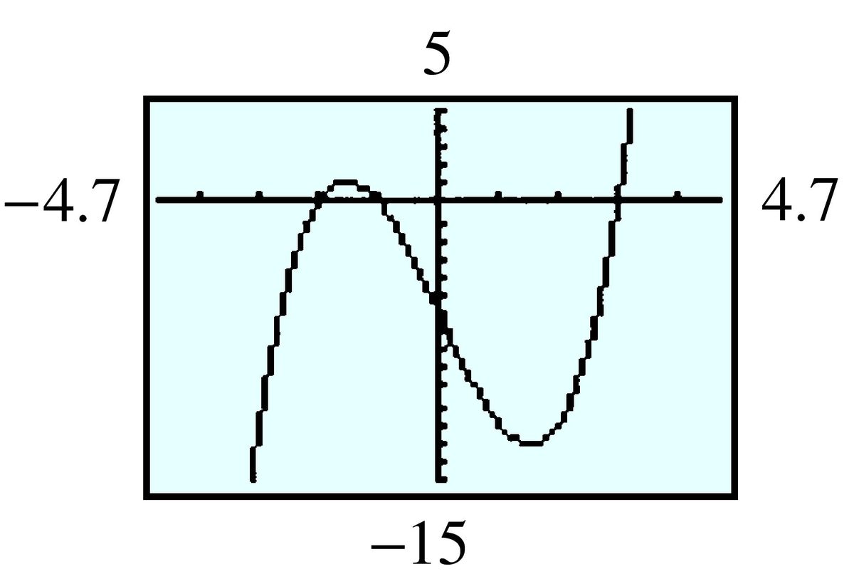
- Yes
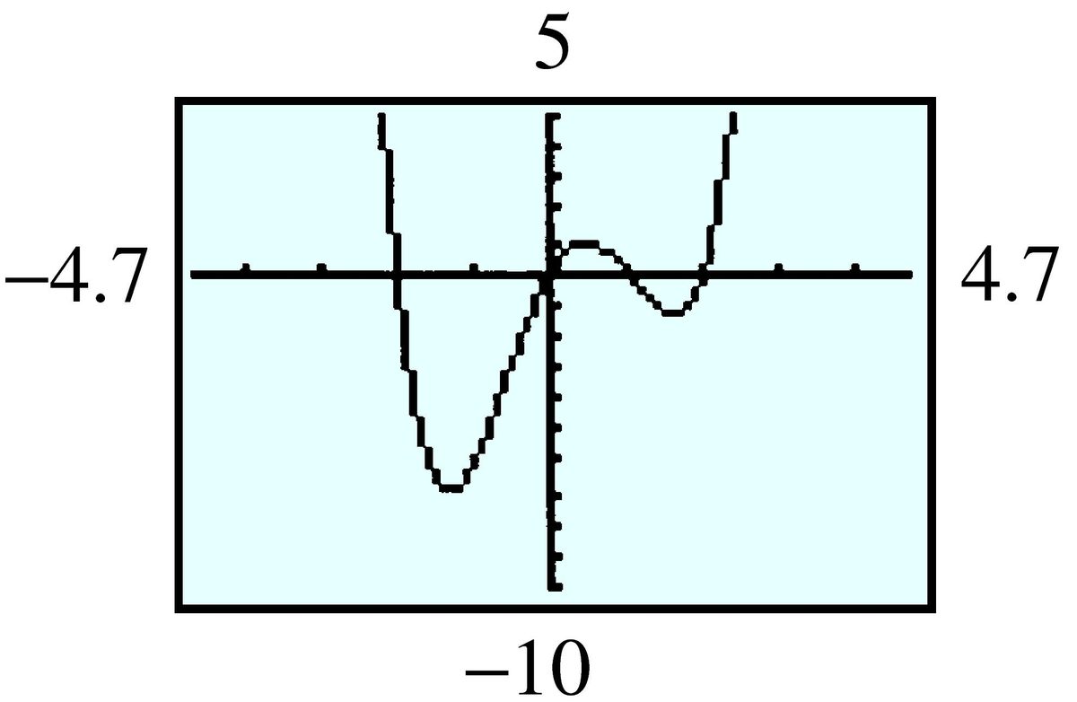
- Yes
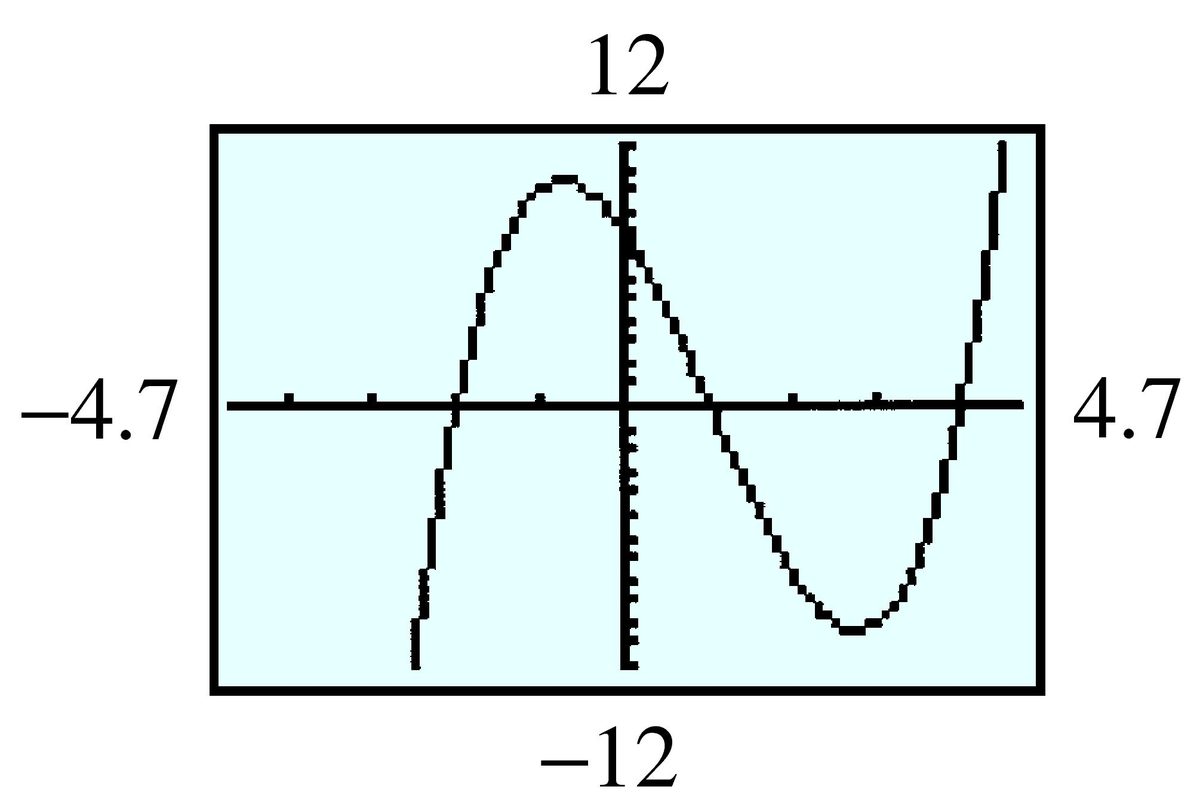
- Yes
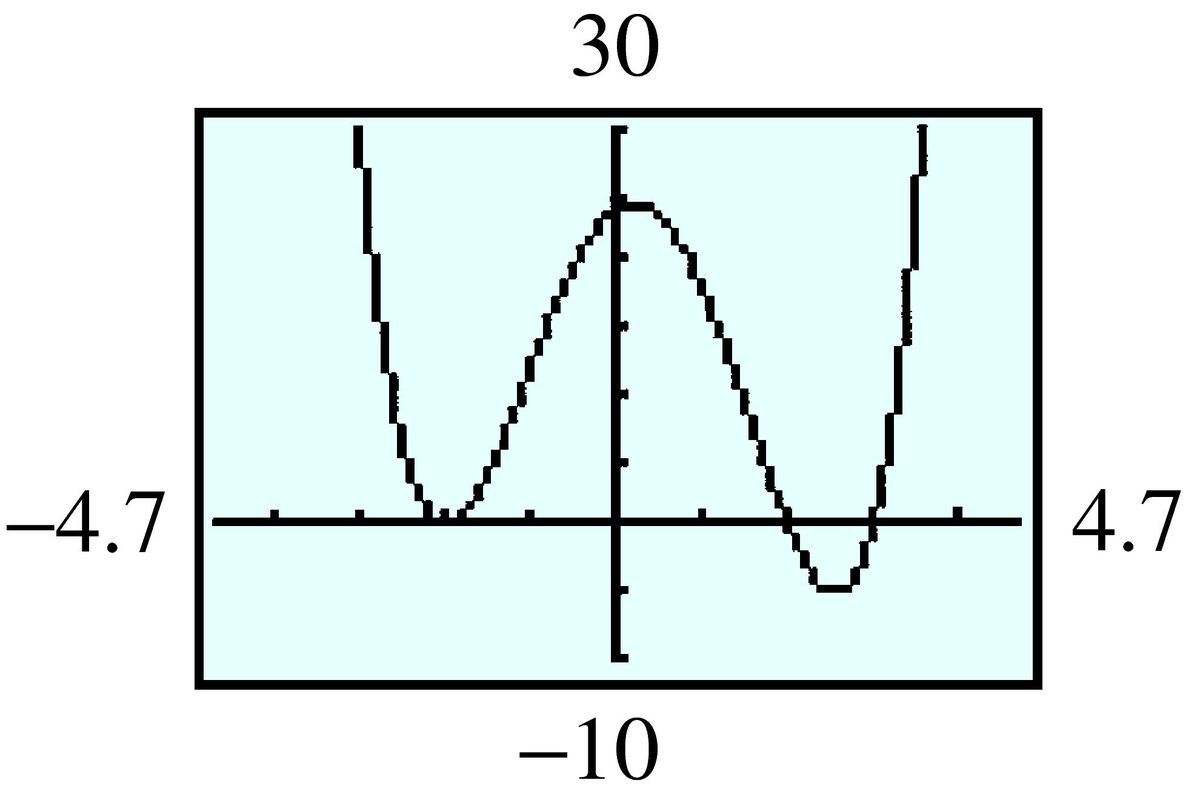
- Yes
For Problems 29–36, sketch a rough graph of each polynomial function by hand, paying attention to the shape of the graph near each -intercept. Check by graphing with a calculator.
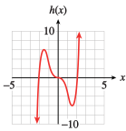
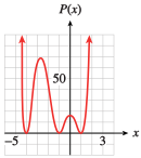
>
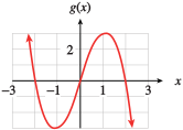
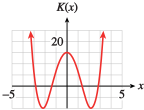
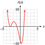
For Problems 37–46,
- Find the zeros of each polynomial by factoring.
- Sketch a rough graph by hand.
- (multiplicity 2)
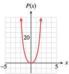
- (multiplicity 2), (multiplicity 2)
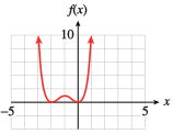
- (multiplicity 2)
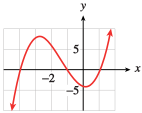
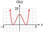
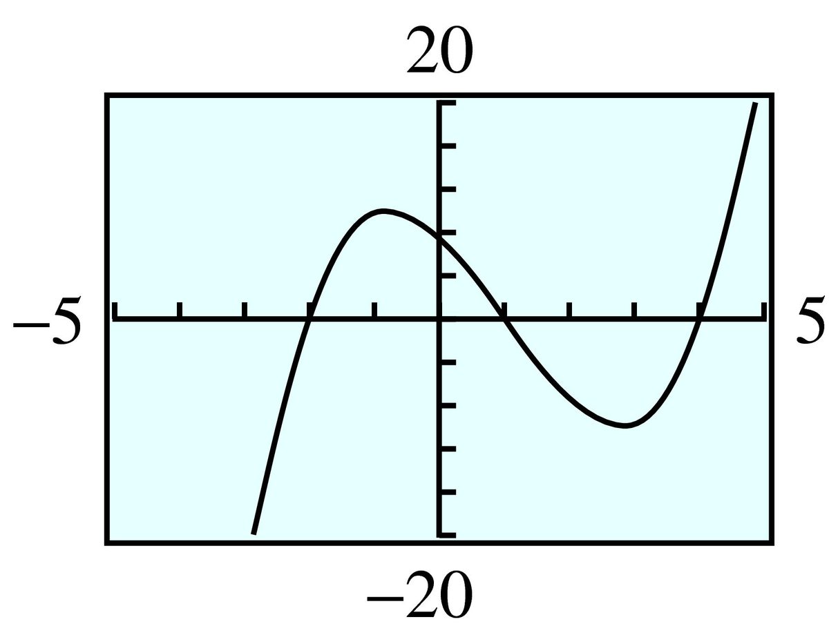
For Problems 47–52, find a possible equation for the polynomial whose graph is shown.
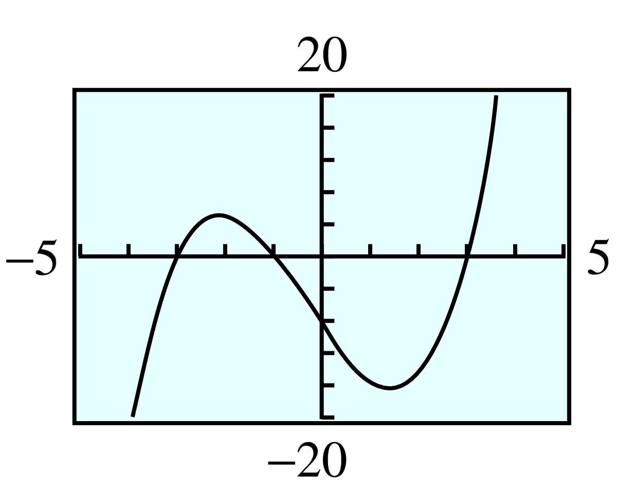
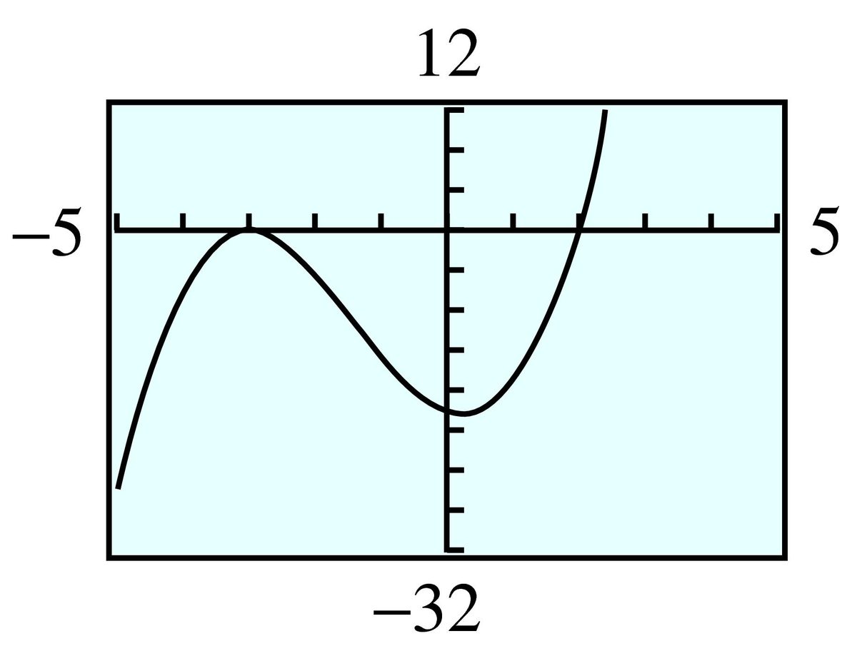
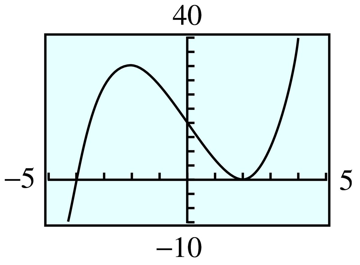
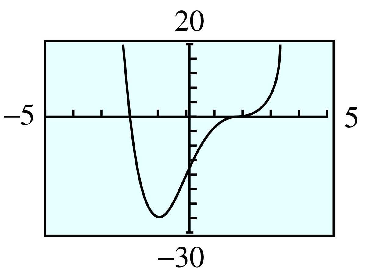
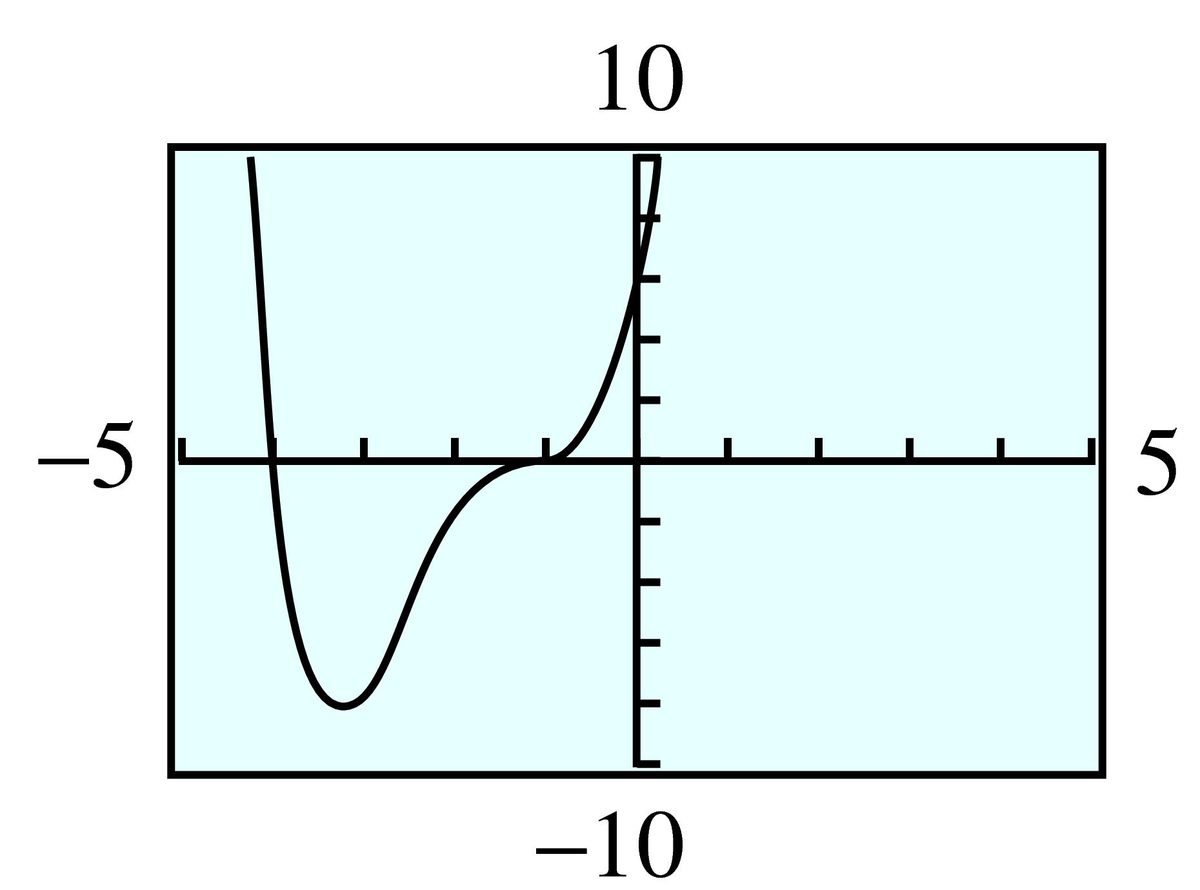
For Problems 53–56, write the formula for each function in parts (a) through (d) and graph with a calculator. Describe how the graph differs from the graph of .
- ; The graph of shifted units up.
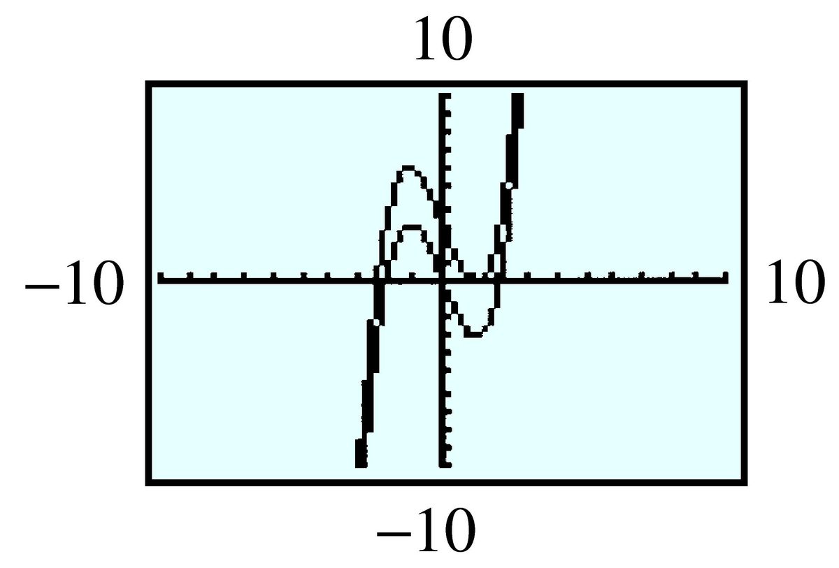
- ; The graph of shifted units down.
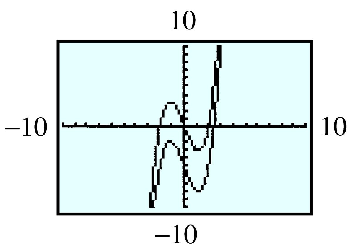
- ; The graph of shifted units right.
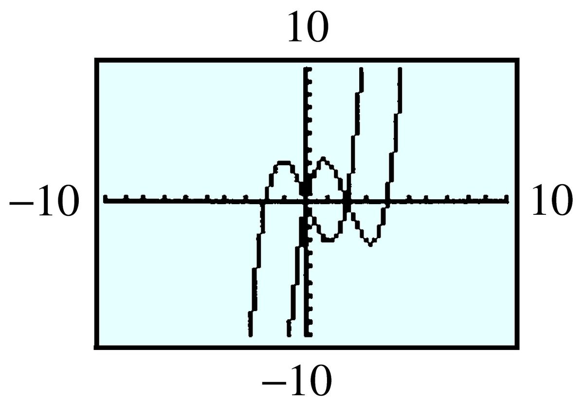
- ; The graph of shifted units left.
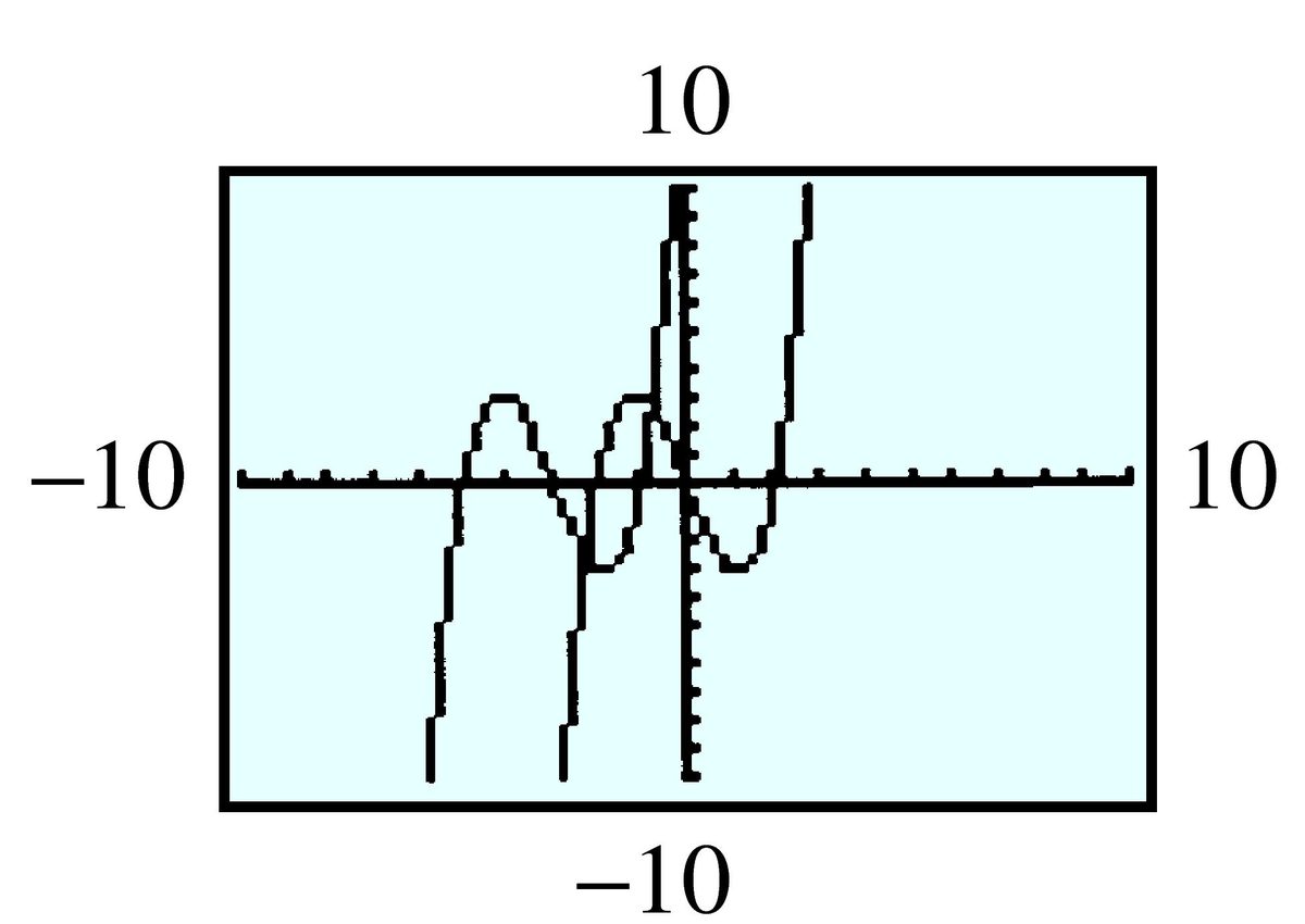
- ; The graph of shifted units up.
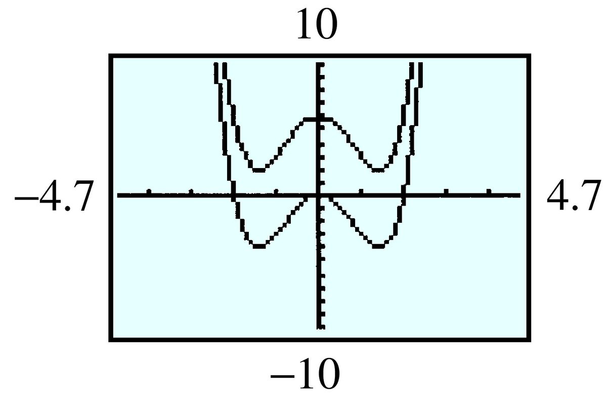
- ; The graph of shifted units down.
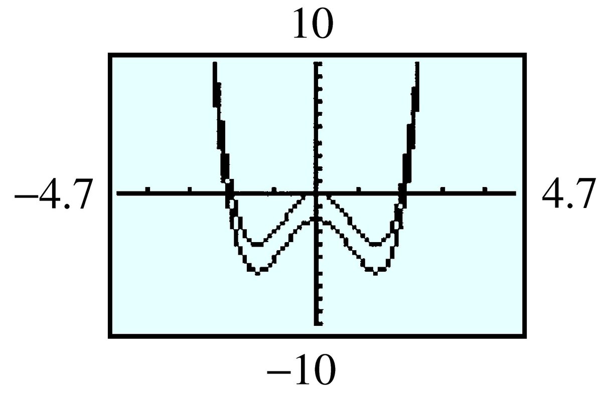
- ; The graph of shifted unit right.
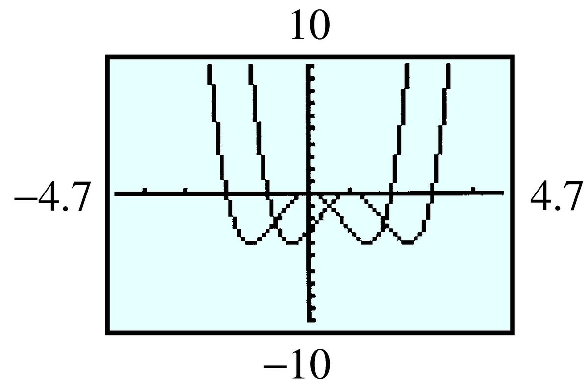
- ; The graph of shifted units left.
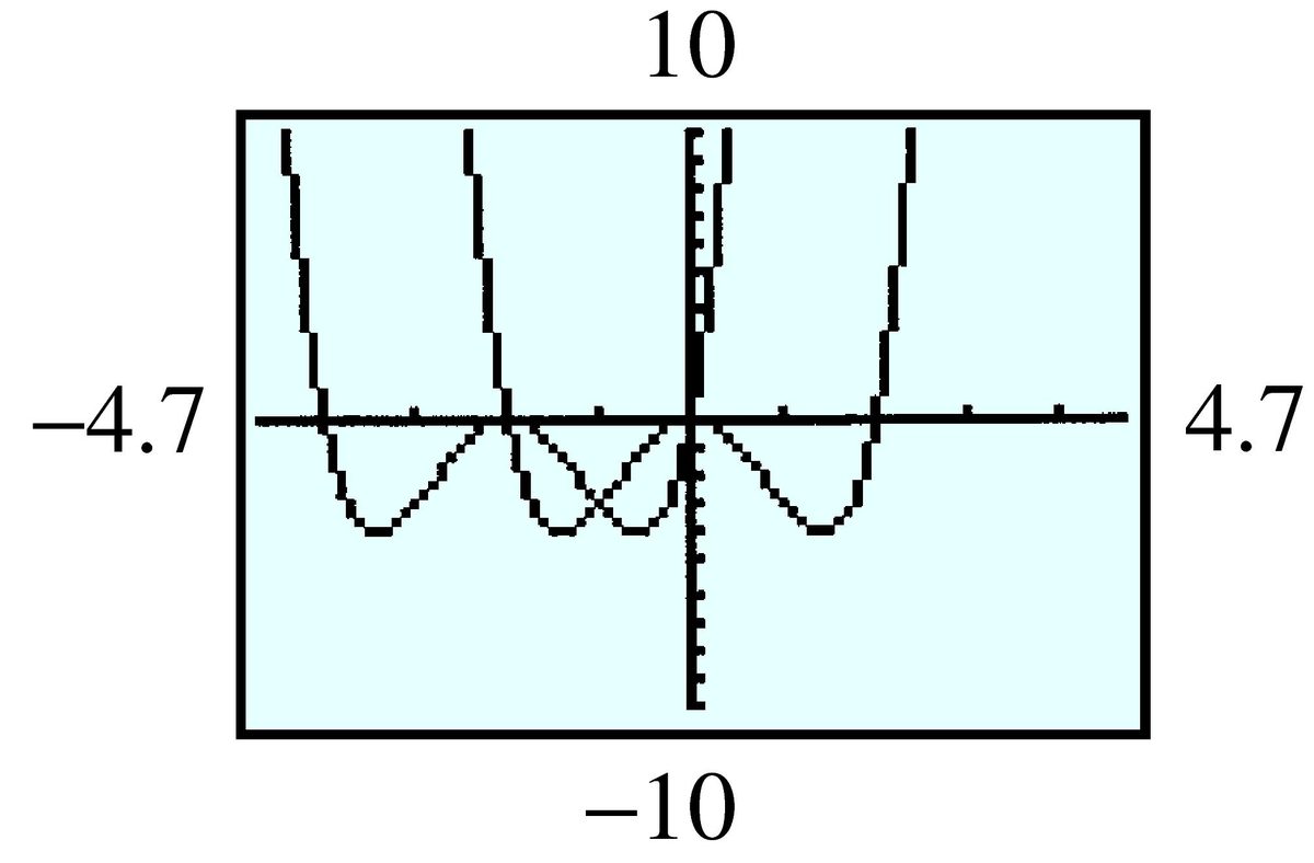
In Problems 57–60, use polynomial division to divide by , and hence find the quotient, , and remainder, . (See Algebra Skills Refresher Polynomials and Factoring to review polynomial division.)
;
;
The remainder theorem states: If is a polynomial and is any real number, there is a unique polynomial such that
Follow the steps below to prove the remainder theorem
- State the division algorithm applied to the polynomials and .
- What must be the degree of in this case?
- Evaluate your expression from part (a) at . What does this tell you about the remainder, ?
- If is a nonconstant polynomial with real coefficients and is any real number, then there exist unique polynomials and such that where .
- Zero
- . Because , is a constant. That constant value is , so .
Verify the remainder theorem for the following:
Use the remainder theorem to prove the factor theorem, stated earlier in this section. You will need to justify two statements:
- If , show that is a factor of .
- If is a factor of , show that .
- From the remainder theorem,
- By definition of a factor, if is a factor of , then , so . The uniqueness guaranteed in the remainder theorem tells us that .
Verify the factor theorem for the following:
For Problems 65–68,
- Verify that the given value is a zero of the polynomial.
- Find the other zeros. (Hint: Use polynomial division to write then factor )
;
;
;
;
In Problems 69–70, we use polynomials to approximate other functions.
- Graph the functions and in the standard window. For what values of does it appear that would be a good approximation for ?
- Change the window settings to
and fill in the table of values below. (You can use the value feature on your calculator.)
- The error in the approximation is the difference . We can reduce the error by using a polynomial of higher degree. The th degree polynomial for approximating is where . Graph and in the same window as in part (b). What is the error in approximating by ?
- Graph in the same window as in part (b). What does the graph tell you about the error in approximating by ?
- About
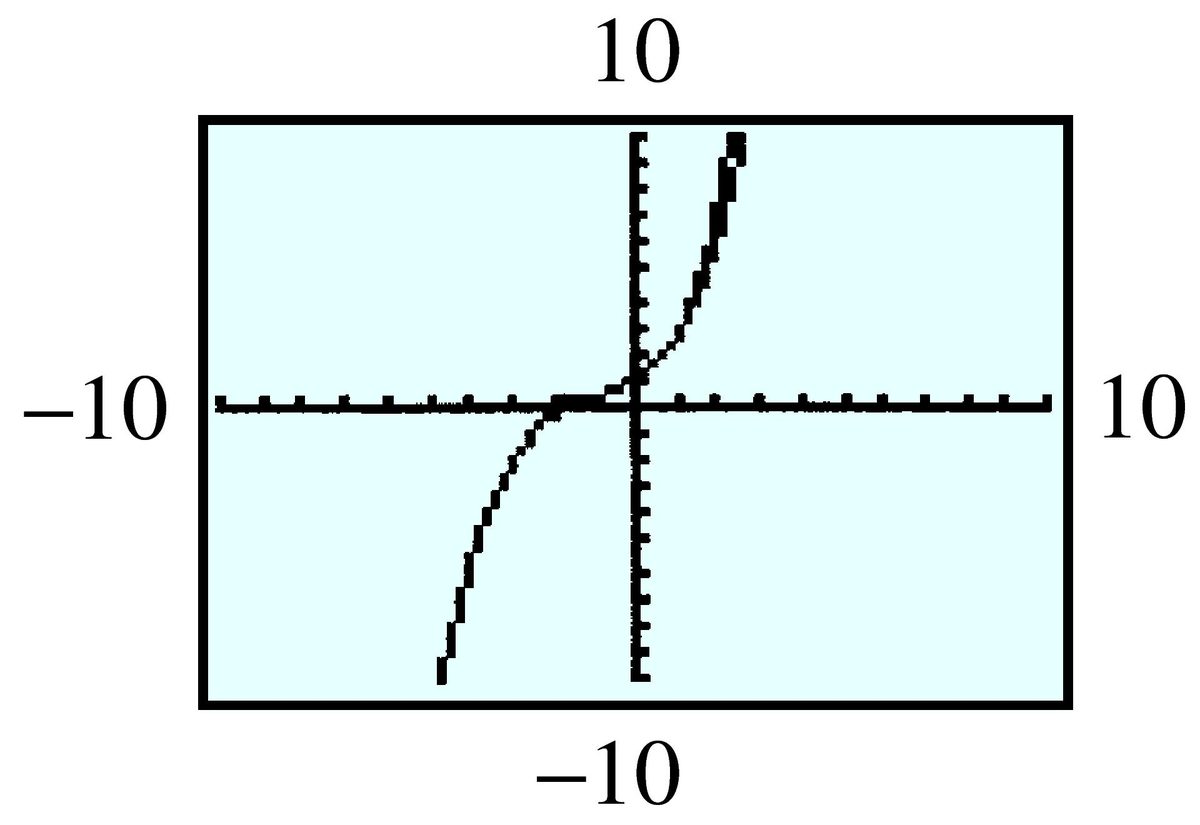
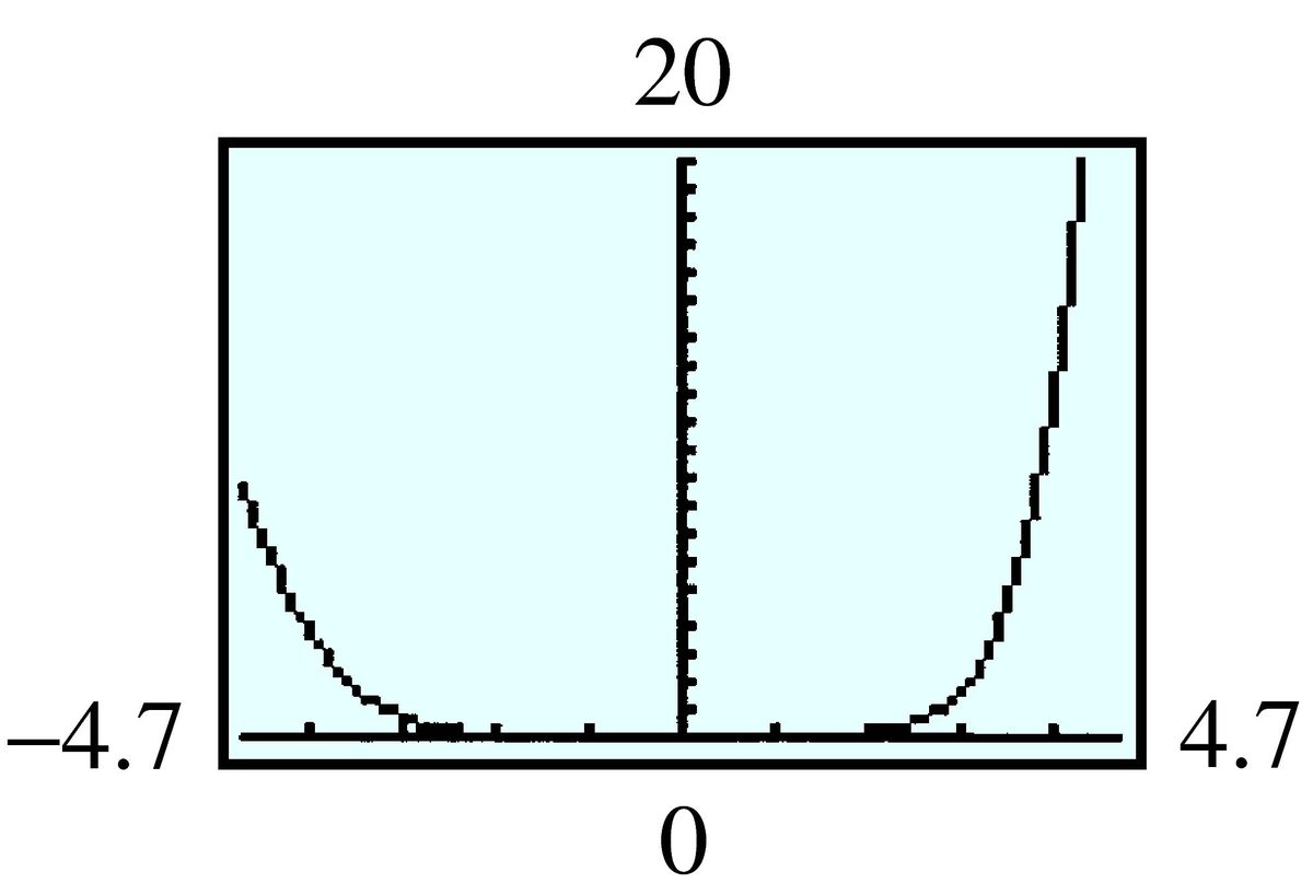
The error is relatively small for values of between and .
In Projects for Chapter 2: Periodic Functions, we investigated periodic functions. The sine function, , is a useful periodic function.
- Graph the functions in the standard window. (Check that your calculator is set in Radian mode.) For what values of does it appear that would be a good approximation for ?
- Change the window settings to
and fill in the table of values below. (You can use the value feature on your calculator.)
- Two more polynomials for approximating are (See Problem for the definition of .) Graph and in the same window as in part (b). What is the error in approximating by ?
- Graph in the same window as in part (b). What does the graph tell you about the error in approximating by ?
Modeling, Functions, and Graphs by Katherine Yoshiwara (yoshiwarabooks.org), GNU Free Documentation License 1.2 or later. Adapted for the XYZ HTML edition with the authors' permission (recorded 2026-07-04). License: GFDL-1.2-or-later.