
1.1 Sets of Real Numbers and the Cartesian Coordinate Plane
Sets of Numbers
While the authors would like nothing more than to delve quickly and deeply into the sheer excitement that is Precalculus, experience1 has taught us that a brief refresher on some basic notions is welcome, if not completely necessary, at this stage. To that end, we present a brief summary of `set theory' and some of the associated vocabulary and notations we use in the text. Like all good Math books, we begin with a definition.
For example, the collection of letters that make up the word “smolko” is well-defined and is a set, but the collection of the worst math teachers in the world is not well-defined, and so is not a set.2 In general, there are three ways to describe sets. They are
Ways to Describe Sets
- The Verbal Method: Use a sentence to define a set.
- The Roster Method: Begin with a left brace `', list each element of the set only once and then end with a right brace `'.
- The Set-Builder Method: A combination of the verbal and roster methods using a “dummy variable” such as .
For example, let be the set described verbally as the set of letters that make up the word “smolko”. A roster description of would be . Note that we listed `o' only once, even though it appears twice in “smolko.” Also, the order of the elements doesn't matter, so is also a roster description of . A set-builder description of is:
The way to read this is: `The set of elements such that is a letter in the word “smolko.”' In each of the above cases, we may use the familiar equals sign `' and write or . Clearly is in and is not in . We express these sentiments mathematically by writing and . Throughout your mathematical upbringing, you have encountered several famous sets of numbers. They are listed below.
Sets of Numbers
- The Empty Set: . This is the set with no elements. Like the number `,' it plays a vital role in mathematics.3
- The Natural Numbers: The periods of ellipsis here indicate that the natural numbers contain , , , `and so forth'.
- The Whole Numbers:
- The Integers:
The Rational Numbers: . Rational numbers are the ratios of integers (provided the denominator is not zero!) It turns out that another way to describe the rational numbers4 is:
- The Real Numbers:
- The Irrational Numbers: Said another way, an irrational number is a decimal which neither repeats nor terminates.5
- The Complex Numbers: Despite their importance, the complex numbers play only a minor role in the text.6
It is important to note that every natural number is a whole number, which, in turn, is an integer. Each integer is a rational number (take in the above definition for ) and the rational numbers are all real numbers, since they possess decimal representations.7 If we take in the above definition of , we see that every real number is a complex number. In this sense, the sets , , , , , and are `nested' like Matryoshka dolls .
For the most part, this textbook focuses on sets whose elements come from the real numbers . Recall that we may visualize as a line. Segments of this line are called intervals of numbers. Below is a summary of the so-called interval notation associated with given sets of numbers. For intervals with finite endpoints, we list the left endpoint, then the right endpoint. We use square brackets, `' or `', if the endpoint is included in the interval and use a filled-in or `closed' dot to indicate membership in the interval. Otherwise, we use parentheses, `' or `' and an `open' circle to indicate that the endpoint is not part of the set. If the interval does not have finite endpoints, we use the symbols to indicate that the interval extends indefinitely to the left and to indicate that the interval extends indefinitely to the right. Since infinity is a concept, and not a number, we always use parentheses when using these symbols in interval notation, and use an appropriate arrow to indicate that the interval extends indefinitely in one (or both) directions.
Interval Notation
Let and be real numbers with .
Set of Real Numbers
Interval Notation
Region on the Real Number Line


For an example, consider the sets of real numbers described below.
Set of Real Numbers
Interval Notation
Region on the Real Number Line


We will often have occasion to combine sets. There are two basic ways to combine sets: intersection and union. We define both of these concepts below.
Said differently, the intersection of two sets is the overlap of the two sets – the elements which the sets have in common. The union of two sets consists of the totality of the elements in each of the sets, collected together.8 For example, if and , then and . If and , then we can find and graphically. To find , we shade the overlap of the two and obtain . To find , we shade each of and and describe the resulting shaded region to find .
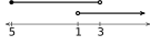
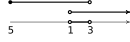
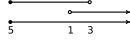
While both intersection and union are important, we have more occasion to use union in this text than intersection, simply because most of the sets of real numbers we will be working with are either intervals or are unions of intervals, as the following example illustrates.
The Cartesian Coordinate Plane
In order to visualize the pure excitement that is Precalculus, we need to unite Algebra and Geometry. Simply put, we must find a way to draw algebraic things. Let's start with possibly the greatest mathematical achievement of all time: the Cartesian Coordinate Plane.9 Imagine two real number lines crossing at a right angle at as drawn below.
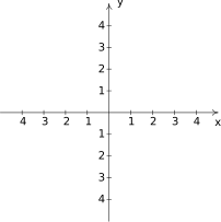
The horizontal number line is usually called the -axis while the vertical number line is usually called the -axis.10 As with the usual number line, we imagine these axes extending off indefinitely in both directions.11 Having two number lines allows us to locate the positions of points off of the number lines as well as points on the lines themselves.
For example, consider the point on the next page. To use the numbers on the axes to label this point, we imagine dropping a vertical line from the -axis to and extending a horizontal line from the -axis to . This process is sometimes called `projecting' the point to the - (respectively -) axis. We then describe the point using the ordered pair . The first number in the ordered pair is called the abscissa or -coordinate and the second is called the ordinate or -coordinate.12 Taken together, the ordered pair comprise the Cartesian coordinates 13 of the point . In practice, the distinction between a point and its coordinates is blurred; for example, we often speak of `the point .' We can think of as instructions on how to reach from the origin by moving units to the right and units downwards. Notice that the order in the ordered pair is important if we wish to plot the point , we would move to the left units from the origin and then move upwards units, as below on the right.
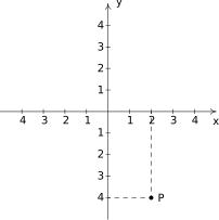
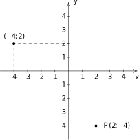
When we speak of the Cartesian Coordinate Plane, we mean the set of all possible ordered pairs as and take values from the real numbers. Below is a summary of important facts about Cartesian coordinates.
Important Facts about the Cartesian Coordinate Plane
- and represent the same point in the plane if and only if and .
- lies on the -axis if and only if .
- lies on the -axis if and only if .
- The origin is the point . It is the only point common to both axes.
The axes divide the plane into four regions called quadrants. They are labeled with Roman numerals and proceed counterclockwise around the plane:
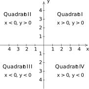
For example, lies in Quadrant I, in Quadrant II, in Quadrant III and in Quadrant IV. If a point other than the origin happens to lie on the axes, we typically refer to that point as lying on the positive or negative -axis (if ) or on the positive or negative -axis (if ). For example, lies on the positive -axis whereas lies on the negative -axis. Such points do not belong to any of the four quadrants.
One of the most important concepts in all of Mathematics is symmetry.15 There are many types of symmetry in Mathematics, but three of them can be discussed easily using Cartesian Coordinates.
Schematically,
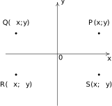
In the above figure, and are symmetric about the -axis, as are and ; and are symmetric about the -axis, as are and ; and and are symmetric about the origin, as are and .
One way to visualize the processes in the previous example is with the concept of a reflection. If we start with our point and pretend that the -axis is a mirror, then the reflection of across the -axis would lie at . If we pretend that the -axis is a mirror, the reflection of across that axis would be . If we reflect across the -axis and then the -axis, we would go from to then to , and so we would end up at the point symmetric to about the origin. We summarize and generalize this process below.
Reflections
To reflect a point about the:
- -axis, replace with .
- -axis, replace with .
- origin, replace with and with .
Distance in the Plane
Another important concept in Geometry is the notion of length. If we are going to unite Algebra and Geometry using the Cartesian Plane, then we need to develop an algebraic understanding of what distance in the plane means. Suppose we have two points, and in the plane. By the distance between and , we mean the length of the line segment joining with . (Remember, given any two distinct points in the plane, there is a unique line containing both points.) Our goal now is to create an algebraic formula to compute the distance between these two points. Consider the generic situation below on the left.
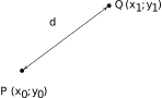
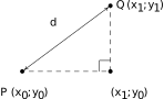
With a little more imagination, we can envision a right triangle whose hypotenuse has length as drawn above on the right. From the latter figure, we see that the lengths of the legs of the triangle are and so the Pythagorean Theorem gives us
(Do you remember why we can replace the absolute value notation with parentheses?) By extracting the square root of both sides of the second equation and using the fact that distance is never negative, we get
It is not always the case that the points and lend themselves to constructing such a triangle. If the points and are arranged vertically or horizontally, or describe the exact same point, we cannot use the above geometric argument to derive the distance formula. It is left to the reader in Exercise to verify Equation for these cases.
Related to finding the distance between two points is the problem of finding the midpoint of the line segment connecting two points. Given two points, and , the midpoint of and is defined to be the point on the line segment connecting and whose distance from is equal to its distance from .
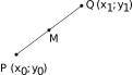
If we think of reaching by going `halfway over' and `halfway up' we get the following formula.
If we let denote the distance between and , we leave it as Exercise to show that the distance between and is which is the same as the distance between and . This suffices to show that Equation gives the coordinates of the midpoint.
We close with a more abstract application of the Midpoint Formula. We will revisit the following example in Exercise in Section.
Exercises
Fill in the chart below:
Set of Real Numbers
Interval Notation
Region on the Real Number Line

Figure 1.32 
Figure 1.33 
Figure 1.34 Plot and label the points , , , , , , and in the Cartesian Coordinate Plane given below.
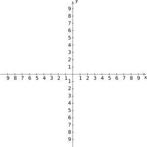
Figure 1.35 For each point given in Exercise above
- Identify the quadrant or axis in/on which the point lies.
- Find the point symmetric to the given point about the -axis.
- Find the point symmetric to the given point about the -axis.
- Find the point symmetric to the given point about the origin.
- ,
- ,
- ,
- ,
- , .
- ,
- , .
- ,
- Find all of the points of the form which are units from the point .
- Find all of the points on the -axis which are units from the point .
- Find all of the points on the -axis which are units from the point .
- Find all of the points of the form which are unit from the origin.
- Let's assume for a moment that we are standing at the origin and the positive -axis points due North while the positive -axis points due East. Our Sasquatch-o-meter tells us that Sasquatch is 3 miles West and 4 miles South of our current position. What are the coordinates of his position? How far away is he from us? If he runs 7 miles due East what would his new position be?
Verify the Distance Formula for the cases when:
- The points are arranged vertically. (Hint: Use and .)
- The points are arranged horizontally. (Hint: Use and .)
- The points are actually the same point. (You shouldn't need a hint for this one.)
- Verify the Midpoint Formula by showing the distance between and and the distance between and are both half of the distance between and .
Show that the points , and below are the vertices of a right triangle.
- , , and
- , and
- Find a point such that the points , , and are the corners of a square. Justify your answer.
- Discuss with your classmates how many numbers are in the interval .
- The world is not flat.16 Thus the Cartesian Plane cannot possibly be the end of the story. Discuss with your classmates how you would extend Cartesian Coordinates to represent the three dimensional world. What would the Distance and Midpoint formulas look like, assuming those concepts make sense at all?
In Exercises -, find the indicated intersection or union and simplify if possible. Express your answers in interval notation.
In Exercises -, write the set using interval notation.
In Exercises -, find the distance between the points and the midpoint of the line segment which connects them.
Answers
Set of Real Numbers
Interval Notation
Region on the Real Number Line

Figure 1.36 
Figure 1.37 
Figure 1.38 
Figure 1.39 
Figure 1.40 
Figure 1.41 
Figure 1.42 
Figure 1.43 
Figure 1.44 
Figure 1.45 The required points , , , , , , , and are plotted in the Cartesian Coordinate Plane below.
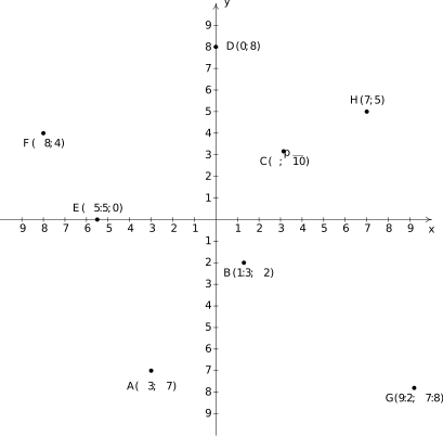
Figure 1.46 The point is
- in Quadrant III
- symmetric about -axis with
- symmetric about -axis with
- symmetric about origin with
The point is
- in Quadrant IV
- symmetric about -axis with
- symmetric about -axis with
- symmetric about origin with
The point is
- in Quadrant I
- symmetric about -axis with
- symmetric about -axis with
- symmetric about origin with
The point is
- on the positive -axis
- symmetric about -axis with
- symmetric about -axis with
- symmetric about origin with
The point is
- on the negative -axis
- symmetric about -axis with
- symmetric about -axis with
- symmetric about origin with
The point is
- in Quadrant II
- symmetric about -axis with
- symmetric about -axis with
- symmetric about origin with
The point is
- in Quadrant IV
- symmetric about -axis with
- symmetric about -axis with
- symmetric about origin with
The point is
- in Quadrant I
- symmetric about -axis with
- symmetric about -axis with
- symmetric about origin with
- ,
- ,
- ,
- ,
- ,
- ,
- ,
- ,
- ,
- ,
- ,
- , miles,
- The distance from to is , the distance from to is , and the distance from to is . Since , we are guaranteed by the converse of the Pythagorean Theorem that the triangle is a right triangle.
- Show that
Adapted from Precalculus, 3rd corrected edition, by Carl Stitz and Jeff Zeager (stitz-zeager.com), licensed under CC BY-NC-SA 3.0. Changes were made: reformatted as an accessible XYZ web edition. License: CC-BY-NC-SA-3.0.