
1.7 Transformations
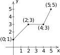
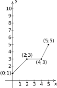
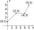
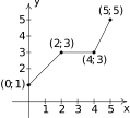
In this section, we study how the graphs of functions change, or transform, when certain specialized modifications are made to their formulas. The transformations we will study fall into three broad categories: shifts, reflections and scalings, and we will present them in that order. Suppose the graph below is the complete graph of a function .
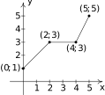
The Fundamental Graphing Principle for Functions says that for a point to be on the graph, . In particular, we know , , and . Suppose we wanted to graph the function defined by the formula . Let's take a minute to remind ourselves of what is doing. We start with an input to the function and we obtain the output . The function takes the output and adds to it. In order to graph , we need to graph the points . How are we to find the values for without a formula for ? The answer is that we don't need a formula for , we just need the values of . The values of are the values on the graph of . For example, using the points indicated on the graph of , we can make the following table.
In general, if is on the graph of , then , so . Hence, is on the graph of . In other words, to obtain the graph of , we add to the -coordinate of each point on the graph of . Geometrically, adding to the -coordinate of a point moves the point units above its previous location. Adding to every -coordinate on a graph en masse is usually described as `shifting the graph up units'. Notice that the graph retains the same basic shape as before, it is just units above its original location. In other words, we connect the four points we moved in the same manner in which they were connected before. We have the results side-by-side at the top of the next page.
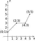
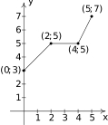
You'll note that the domain of and the domain of are the same, namely , but that the range of is while the range of is . In general, shifting a function vertically like this will leave the domain unchanged, but could very well affect the range. You can easily imagine what would happen if we wanted to graph the function . Instead of adding to each of the -coordinates on the graph of , we'd be subtracting . Geometrically, we would be moving the graph down units. We leave it to the reader to verify that the domain of is the same as , but the range of is . What we have discussed is generalized in the following theorem.
The key to understanding Theorem 1.2 and, indeed, all of the theorems in this section comes from an understanding of the Fundamental Graphing Principle for Functions. If is on the graph of , then . Substituting into the equation gives . Hence, is on the graph of , and we have the result. In the language of `inputs' and `outputs', Theorem 1.2 can be paraphrased as “Adding to, or subtracting from, the output of a function causes the graph to shift up or down, respectively.” So what happens if we add to or subtract from the input of the function?
Keeping with the graph of above, suppose we wanted to graph . In other words, we are looking to see what happens when we add to the input of the function.1 Let's try to generate a table of values of based on those we know for . We quickly find that we run into some difficulties.
When we substitute into the formula , we are asked to find which doesn't exist because the domain of is only . The same thing happens when we attempt to find . What we need here is a new strategy. We know, for instance, . To determine the corresponding point on the graph of , we need to figure out what value of we must substitute into so that the quantity , works out to be . Solving gives , and so is on the graph of . To use the fact , we set to get . Substituting gives . Continuing in this fashion, we get
In summary, the points , , and on the graph of give rise to the points , , and on the graph of , respectively. In general, if is on the graph of , then . Solving gives so that . As such, is on the graph of . The point is exactly units to the left of the point so the graph of is obtained by shifting the graph to the left units, as pictured below.
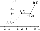
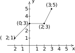
Note that while the ranges of and are the same, the domain of is whereas the domain of is . In general, when we shift the graph horizontally, the range will remain the same, but the domain could change. If we set out to graph , we would find ourselves adding to all of the values of the points on the graph of to effect a shift to the right units. Generalizing these notions produces the following result.
In other words, Theorem 1.3 says that adding to or subtracting from the input to a function amounts to shifting the graph left or right, respectively. Theorems 1.2 and 1.3 present a theme which will run common throughout the section: changes to the outputs from a function affect the -coordinates of the graph, resulting in some kind of vertical change; changes to the inputs to a function affect the -coordinates of the graph, resulting in some kind of horizontal change.
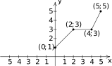
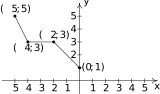
We now turn our attention to reflections. We know from Section 1.1 that to reflect a point across the -axis, we replace with . If is on the graph of , then , so replacing with is the same as replacing with . Hence, the graph of is the graph of reflected across the -axis. Similarly, the graph of is the graph of reflected across the -axis. Returning to the language of inputs and outputs, multiplying the output from a function by reflects its graph across the -axis, while multiplying the input to a function by reflects the graph across the -axis.4
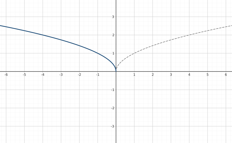
Applying Theorem 1.4 to the graph of given at the beginning of the section, we can graph by reflecting the graph of about the -axis
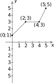
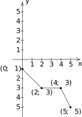
By reflecting the graph of across the -axis, we obtain the graph of .
With the addition of reflections, it is now more important than ever to consider the order of transformations, as the next example illustrates.
We now turn our attention to our last class of transformations known as scalings. A thorough discussion of scalings can get complicated because they are not as straight-forward as the previous transformations. A quick review of what we've covered so far, namely vertical shifts, horizontal shifts and reflections, will show you why those transformations are known as rigid transformations. Simply put, they do not change the shape of the graph, only its position and orientation in the plane. If, however, we wanted to make a new graph twice as tall as a given graph, or one-third as wide, we would be changing the shape of the graph. This type of transformation is called non-rigid for obvious reasons. Not only will it be important for us to differentiate between modifying inputs versus outputs, we must also pay close attention to the magnitude of the changes we make. As you will see shortly, the Mathematics turns out to be easier than the associated grammar.
Suppose we wish to graph the function where is the function whose graph is given at the beginning of the section. From its graph, we can build a table of values for as before.
In general, if is on the graph of , then so that puts on the graph of . In other words, to obtain the graph of , we multiply all of the -coordinates of the points on the graph of by . Multiplying all of the -coordinates of all of the points on the graph of by causes what is known as a `vertical scaling7 by a factor of ', and the results are given on the next page.
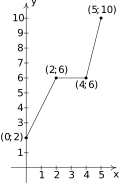
If we wish to graph , we multiply the all of the -coordinates of the points on the graph of by . This creates a `vertical scaling8 by a factor of ' as seen below.
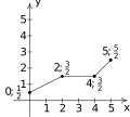
These results are generalized in the following theorem.
A few remarks about Theorem 1.5 are in order. First, a note about the verbiage. To the authors, the words `stretching', `expansion', and `dilation' all indicate something getting bigger. Hence, `stretched by a factor of ' makes sense if we are scaling something by multiplying it by . Similarly, we believe words like `shrinking', `compression' and `contraction' all indicate something getting smaller, so if we scale something by a factor of , we would say it `shrinks by a factor of ' - not `shrinks by a factor of '. This is why we have written the descriptions `stretching by a factor of ' and `shrinking by a factor of ' in the statement of the theorem. Second, in terms of inputs and outputs, Theorem 1.5 says multiplying the outputs from a function by positive number causes the graph to be vertically scaled by a factor of . It is natural to ask what would happen if we multiply the inputs of a function by a positive number. This leads us to our last transformation of the section.
Referring to the graph of given at the beginning of this section, suppose we want to graph . In other words, we are looking to see what effect multiplying the inputs to by has on its graph. If we attempt to build a table directly, we quickly run into the same problem we had in our discussion leading up to Theorem 1.3, as seen in the table on the left below. We solve this problem in the same way we solved this problem before. For example, if we want to determine the point on which corresponds to the point on the graph of , we set so that . Substituting into , we obtain , so that is on the graph of . Continuing in this fashion, we obtain the table on the lower right.
In general, if is on the graph of , then . Hence so that is on the graph of . In other words, to graph we divide the -coordinates of the points on the graph of by . This results in a horizontal scaling9 by a factor of .
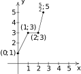
If, on the other hand, we wish to graph , we end up multiplying the -coordinates of the points on the graph of by which results in a horizontal scaling10 by a factor of , as demonstrated below.
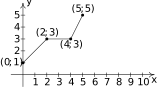
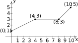
We have the following theorem.
Theorem 1.6 tells us that if we multiply the input to a function by , the resulting graph is scaled horizontally by a factor of since the -values are divided by to produce corresponding points on the graph of . The next example explores how vertical and horizontal scalings sometimes interact with each other and with the other transformations introduced in this section.
Some comments about Example 1.7.3 are in order. First, recalling the properties of radicals from Intermediate Algebra, we know that the functions and are the same, since and have the same domains and . (We invite the reader to verify that all of the points we plotted on the graph of lie on the graph of and vice-versa.) Hence, for , a vertical stretch by a factor of and a horizontal shrinking by a factor of result in the same transformation. While this kind of phenomenon is not universal, it happens commonly enough with some of the families of functions studied in College Algebra that it is worthy of note. Secondly, to graph the function , we applied a series of four transformations. While it would have been easier on the authors to simply inform the reader of which steps to take, we have strived to explain why the order in which the transformations were applied made sense. We generalize the procedure in the theorem below.
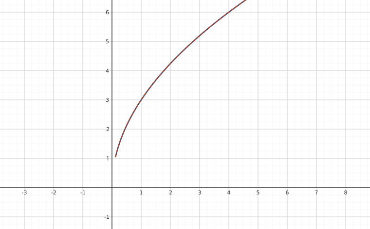
Theorem 1.7 can be established by generalizing the techniques developed in this section. Suppose is on the graph of . Then , and to make good use of this fact, we set and solve. We first subtract the (causing the horizontal shift) and then divide by . If is a positive number, this induces only a horizontal scaling by a factor of . If , then we have a factor of in play, and dividing by it induces a reflection about the -axis. So we have as the input to which corresponds to the input to . We now evaluate . We notice that the output from is first multiplied by . As with the constant , if , this induces only a vertical scaling. If , then the induces a reflection across the -axis. Finally, we add to the result, which is our vertical shift. A less precise, but more intuitive way to paraphrase Theorem 1.7 is to think of the quantity is the `inside' of the function . What's happening inside affects the inputs or -coordinates of the points on the graph of . To find the -coordinates of the corresponding points on , we undo what has been done to in the same way we would solve an equation. What's happening to the output can be thought of as things happening `outside' the function, . Things happening outside affect the outputs or -coordinates of the points on the graph of . Here, we follow the usual order of operations agreement: we first multiply by then add to find the corresponding -coordinates on the graph of .
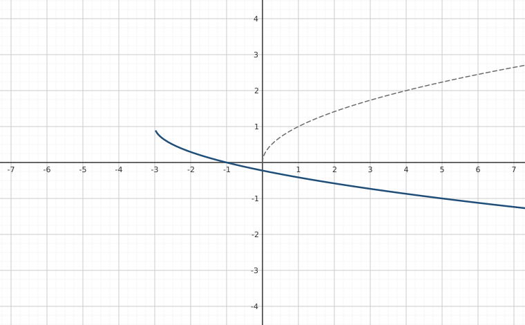
Our last example turns the tables and asks for the formula of a function given a desired sequence of transformations. If nothing else, it is a good review of function notation.
We have kept the viewing window the same in all of the graphs above. This had the undesirable consequence of making the last graph look `incomplete' in that we cannot see the original shape of . Altering the viewing window results in a more complete graph of the transformed function as seen below.
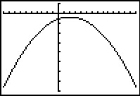
This example brings our first chapter to a close. In the chapters which lie ahead, be on the lookout for the concepts developed here to resurface as we study different families of functions.
Exercises
Suppose is on the graph of . In Exercises -, use Theorem 1.7 to find a point on the graph of the given transformed function.
The complete graph of is given below. In Exercises -, use it and Theorem 1.7 to graph the given transformed function.
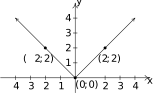
- Some of the answers to Exercises - above should be the same. Which ones match up? What properties of the graph of contribute to the duplication?
The complete graph of is given below. In Exercises -, use it and Theorem 1.7 to graph the given transformed function.
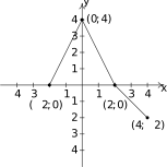
The complete graph of is given below. In Exercises -, use it and Theorem 1.7 to graph the given transformed function.
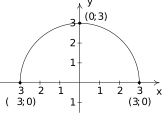
The complete graph of is given below.
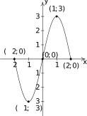
The purpose of Exercises - is to graph by graphing each transformation, one step at a time.
Let . Find a formula for a function whose graph is obtained from from the given sequence of transformations.
- (1) shift right 2 units; (2) shift down 3 units
- (1) shift down 3 units; (2) shift right 2 units
- (1) reflect across the -axis; (2) shift up 1 unit
- (1) shift up 1 unit; (2) reflect across the -axis
- (1) shift left 1 unit; (2) reflect across the -axis; (3) shift up 2 units
- (1) reflect across the -axis; (2) shift left 1 unit; (3) shift up 2 units
- (1) shift left 3 units; (2) vertical stretch by a factor of 2; (3) shift down 4 units
- (1) shift left 3 units; (2) shift down 4 units; (3) vertical stretch by a factor of 2
- (1) shift right 3 units; (2) horizontal shrink by a factor of 2; (3) shift up 1 unit
- (1) horizontal shrink by a factor of 2; (2) shift right 3 units; (3) shift up 1 unit
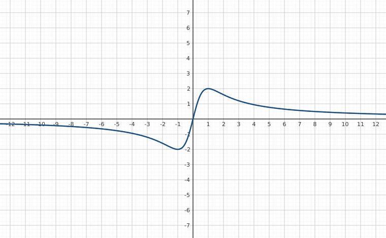
The graph of is given below on the left and the graph of is given on the right. Find a formula for based on transformations of the graph of . Check your answer by confirming that the points shown on the graph of satisfy the equation .
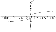
Figure 1.264 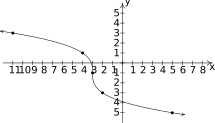
Figure 1.265 - For many common functions, the properties of Algebra make a horizontal scaling the same as a vertical scaling by (possibly) a different factor. For example, we stated earlier that . With the help of your classmates, find the equivalent vertical scaling produced by the horizontal scalings and . What about and ?
- We mentioned earlier in the section that, in general, the order in which transformations are applied matters, yet in our first example with two transformations the order did not matter. (You could perform the shift to the left followed by the shift down or you could shift down and then left to achieve the same result.) With the help of your classmates, determine the situations in which order does matter and those in which it does not.
- What happens if you reflect an even function across the -axis?
- What happens if you reflect an odd function across the -axis?
- What happens if you reflect an even function across the -axis?
- What happens if you reflect an odd function across the -axis?
- How would you describe symmetry about the origin in terms of reflections?
- As we saw in Example 1.7.5, the viewing window on the graphing calculator affects how we see the transformations done to a graph. Using two different calculators, find viewing windows so that on the one calculator looks like on the other.
Answers
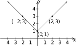
Figure 1.266 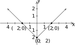
Figure 1.267 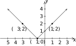
Figure 1.268 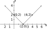
Figure 1.269 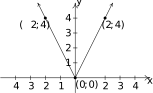
Figure 1.270 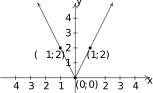
Figure 1.271 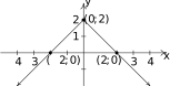
Figure 1.272 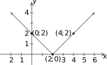
Figure 1.273 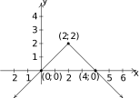
Figure 1.274 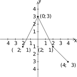
Figure 1.275 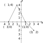
Figure 1.276 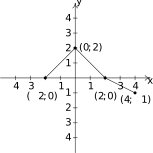
Figure 1.277 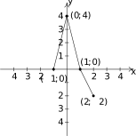
Figure 1.278 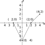
Figure 1.279 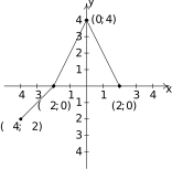
Figure 1.280 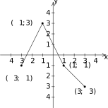
Figure 1.281 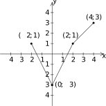
Figure 1.282 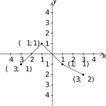
Figure 1.283 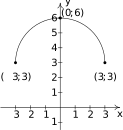
Figure 1.284 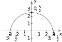
Figure 1.285 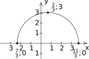
Figure 1.286 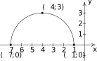
Figure 1.287 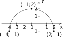
Figure 1.288 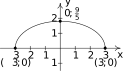
Figure 1.289 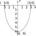
Figure 1.290 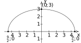
Figure 1.291 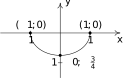
Figure 1.292 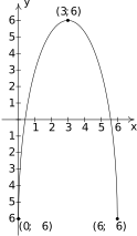
Figure 1.293 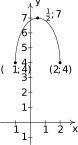
Figure 1.294 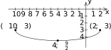
Figure 1.295 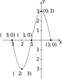
Figure 1.296 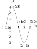
Figure 1.297 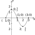
Figure 1.298 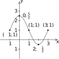
Figure 1.299 - or
Adapted from Precalculus, 3rd corrected edition, by Carl Stitz and Jeff Zeager (stitz-zeager.com), licensed under CC BY-NC-SA 3.0. Changes were made: reformatted as an accessible XYZ web edition. License: CC-BY-NC-SA-3.0.