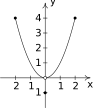
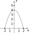
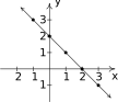
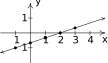
In Section 1.3 we defined a function as a special type of relation; one in which each -coordinate was matched with only one -coordinate. We spent most of our time in that section looking at functions graphically because they were, after all, just sets of points in the plane. Then in Section 1.4 we described a function as a process and defined the notation necessary to work with functions algebraically. So now it's time to look at functions graphically again, only this time we'll do so with the notation defined in Section 1.4. We start with what should not be a surprising connection.
The Fundamental Graphing Principle for Functions
The graph of a function is the set of points which satisfy the equation . That is, the point is on the graph of if and only if .
Graphing piecewise-defined functions is a bit more of a challenge.
In the previous two examples, the -coordinates of the -intercepts of the graph of were found by solving . For this reason, they are called the zeros of .
Of the three symmetries discussed in Section 1.2.1, only two are of significance to functions: symmetry about the -axis and symmetry about the origin.2 Recall that we can test whether the graph of an equation is symmetric about the -axis by replacing with and checking to see if an equivalent equation results. If we are graphing the equation , substituting for results in the equation . In order for this equation to be equivalent to the original equation we need . In a similar fashion, we recall that to test an equation's graph for symmetry about the origin, we replace and with and , respectively. Doing this substitution in the equation results in . Solving the latter equation for gives . In order for this equation to be equivalent to the original equation we need , or, equivalently, . These results are summarized below.
Testing the Graph of a Function for Symmetry
The graph of a function is symmetric
about the -axis if and only if for all in the domain of .
about the origin if and only if for all in the domain of .
For reasons which won't become clear until we study polynomials, we call a function even if its graph is symmetric about the -axis or odd if its graph is symmetric about the origin. Apart from a very specialized family of functions which are both even and odd,3 functions fall into one of three distinct categories: even, odd, or neither even nor odd.
There are two lessons to be learned from the last example. The first is that sampling function values at particular values is not enough to prove that a function is even or odd despite the fact that , turned out not to be odd. Secondly, while the calculator may suggest mathematical truths, it is the Algebra which proves mathematical truths.6
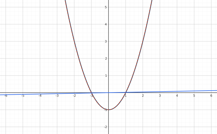
Interactive figureThe calculator trap: j looks even, and is notDrag the Magnification M slider from 1 to 100.
XYZ Graph · viewer build 5edf91b
The trap the example warns about, magnified until it is visible. The solid curve is j(x) = x² − x/100 − 1 and the dashed curve is j(−x): at this scale they sit right on top of one another, which is why a calculator screen suggests j is even. But j(1) = −0.01 while j(−1) = +0.01, so it is not. The straight line through the origin is the difference j(−x) − j(x) = x/50, magnified M times: at M = 1 it is barely distinguishable from the x-axis, but drag M to 100 and the difference is unmistakable — a line of slope 2. If j were even, that difference would be exactly zero for every x and no magnification could lift it off the axis. As the section says: the calculator may suggest mathematical truths, but it is the Algebra which proves them.
General Function Behavior
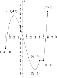
The last topic we wish to address in this section is general function behavior. As you shall see in the next several chapters, each family of functions has its own unique attributes and we will study them all in great detail. The purpose of this section's discussion, then, is to lay the foundation for that further study by investigating aspects of function behavior which apply to all functions. To start, we will examine the concepts of increasing, decreasing and constant. Before defining the concepts algebraically, it is instructive to first look at them graphically. Consider the graph of the function below.
Figure 1.158The graph of
Reading from left to right, the graph `starts' at the point and `ends' at the point . If we imagine walking from left to right on the graph, between and , we are walking `uphill'; then between and , we are walking `downhill'; and between and , we are walking `uphill' once more. From to , we `level off', and then resume walking `uphill' from to . In other words, for the values between and (inclusive), the -coordinates on the graph are getting larger, or increasing, as we move from left to right. Since , the values on the graph are the function values, and we say that the function is increasing on the interval . Analogously, we say that is decreasing on the interval increasing once more on the interval , constant on , and finally increasing once again on . It is extremely important to notice that the behavior (increasing, decreasing or constant) occurs on an interval on the -axis. When we say that the function is increasing on we do not mention the actual values that attains along the way. Thus, we report where the behavior occurs, not to what extent the behavior occurs.7 Also notice that we do not say that a function is increasing, decreasing or constant at a single value. In fact, we would run into serious trouble in our previous example if we tried to do so because is contained in an interval on which was increasing and one on which it is decreasing. (There's more on this issue – and many others – in the Exercises.)
We're now ready for the more formal algebraic definitions of what it means for a function to be increasing, decreasing or constant.
It is worth taking some time to see that the algebraic descriptions of increasing, decreasing and constant as stated in Definition 1.10 agree with our graphical descriptions given earlier. You should look back through the examples and exercise sets in previous sections where graphs were given to see if you can determine the intervals on which the functions are increasing, decreasing or constant. Can you find an example of a function for which none of the concepts in Definition 1.10 apply?
Now let's turn our attention to a few of the points on the graph. Clearly the point does not have the largest value of all of the points on the graph of indeed that honor goes to but should get some sort of consolation prize for being `the top of the hill' between and . We say that the function has a local maximum8 at the point , because the -coordinate is the largest -value (hence, function value) on the curve `near'9
. Similarly, we say that the function has a local minimum10 at the point , since the -coordinate is the smallest function value near . Although it is tempting to say that local extrema11 occur when the function changes from increasing to decreasing or vice versa, it is not a precise enough way to define the concepts for the needs of Calculus. At the risk of being pedantic, we will present the traditional definitions and thoroughly vet the pathologies they induce in the Exercises. We have one last observation to make before we proceed to the algebraic definitions and look at a fairly tame, yet helpful, example.
If we look at the entire graph, we see that the largest value (the largest function value) is at . In this case, we say the maximum12 of is ; similarly, the minimum13 of is .
We formalize these concepts in the following definitions.
It's important to note that not every function will have all of these features. Indeed, it is possible to have a function with no local or absolute extrema at all! (Any ideas of what such a function's graph would have to look like?) We shall see examples of functions in the Exercises which have one or two, but not all, of these features, some that have instances of each type of extremum and some functions that seem to defy common sense. In all cases, though, we shall adhere to the algebraic definitions above as we explore the wonderful diversity of graphs that functions provide us.
Here is the `tame' example which was promised earlier. It summarizes all of the concepts presented in this section as well as some from previous sections so you should spend some time thinking deeply about it before proceeding to the Exercises.
With few exceptions, we will not develop techniques in College Algebra which allow us to determine the intervals on which a function is increasing, decreasing or constant or to find the local maximums and local minimums analytically; this is the business of Calculus.15 When we have need to find such beasts, we will resort to the calculator. Most graphing calculators have `Minimum' and `Maximum' features which can be used to approximate these values, as we now demonstrate.
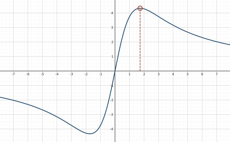
Interactive figureRiding the curve y = 15x/(x² + 3) to its extremaDrag the Probe position c slider from -6 to 6.
XYZ Graph · viewer build 5edf91b
The section's calculator hunt, live: the marked point rides the curve y = 15x/(x² + 3) at x = c, with the dashed rod measuring its height. Drag c and the height climbs as it approaches 1.73 from either side; there the point reads 4.33 to two decimal places — the local maximum the book's calculator approximates — and the mirror-image local minimum of −4.33 sits near c ≈ −1.73: this function is odd, so the two extrema are reflections of each other through the origin. Between −1.73 and 1.73 the curve rises from valley to peak; beyond them it flattens back toward the x-axis on both sides. The intervals of increase and decrease the example reports are exactly what your thumb feels on the slider.
Exercises
In Exercises -, sketch the graph of the given function. State the domain of the function, identify any intercepts and test for symmetry.
In Exercises -, sketch the graph of the given piecewise-defined function.
In Exercises -, determine analytically if the following functions are even, odd or neither.
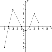
In Exercises -, use the graph of given below to answer the question.
Figure 1.167
Find the domain of .
Find the range of .
Determine .
Solve .
List the -intercepts, if any exist.
List the -intercepts, if any exist.
Find the zeros of .
Solve .
Find the number of solutions to .
Does appear to be even, odd, or neither?
List the intervals where is increasing.
List the intervals where is decreasing.
List the local maximums, if any exist.
List the local minimums, if any exist.
Find the maximum, if it exists.
Find the minimum, if it exists.
In Exercises -, use the graph of given below to answer the question.
Figure 1.168
Find the domain of .
Find the range of .
Determine .
Solve .
List the -intercepts, if any exist.
List the -intercepts, if any exist.
Find the zeros of .
Solve .
Find the number of solutions to .
Does appear to be even, odd, or neither?
List the intervals where is increasing.
List the intervals where is decreasing.
List the local maximums, if any exist.
List the local minimums, if any exist.
Find the maximum, if it exists.
Find the minimum, if it exists.
In Exercises -, use your graphing calculator to approximate the local and absolute extrema of the given function. Approximate the intervals on which the function is increasing and those on which it is decreasing. Round your answers to two decimal places.
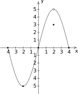
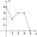
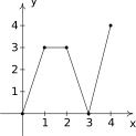
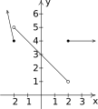
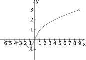
In Exercises -, use the graphs of and below to find the function value.
Figure 1.169Figure 1.170
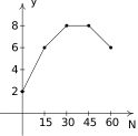
The graph below represents the height of a Sasquatch (in feet) as a function of its age in years. Use it to answer the questions in Exercises -.
Figure 1.171
Find and interpret .
How tall is the Sasquatch when she is 15 years old?
Solve and interpret.
List the interval over which is constant and interpret your answer.
List the interval over which is decreasing and interpret your answer.
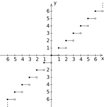
For Exercises -, let be the greatest integer function as defined in Exercise in Section 1.4.
Graph . Be careful to correctly describe the behavior of the graph near the integers.
Is even, odd, or neither? Explain.
Discuss with your classmates which points on the graph are local minimums, local maximums or both. Is ever increasing? Decreasing? Constant?
In Exercises -, use your graphing calculator to show that the given function does not have any extrema, neither local nor absolute.
In Exercise in Section 1.4, we saw that the population of Sasquatch in Portage County could be modeled by the function , where represents the year 1803. Use your graphing calculator to analyze the general function behavior of . Will there ever be a time when 200 Sasquatch roam Portage County?
Suppose and are both even functions. What can be said about the functions , , and ? What if and are both odd? What if is even but is odd?
One of the most important aspects of the Cartesian Coordinate Plane is its ability to put Algebra into geometric terms and Geometry into algebraic terms. We've spent most of this chapter looking at this very phenomenon and now you should spend some time with your classmates reviewing what we've done. What major results do we have that tie Algebra and Geometry together? What concepts from Geometry have we not yet described algebraically? What topics from Intermediate Algebra have we not yet discussed geometrically?
It's now time to “thoroughly vet the pathologies induced” by the precise definitions of local maximum and local minimum. We'll do this by providing you and your classmates a series of Exercises to discuss. You will need to refer back to Definition 1.10 (Increasing, Decreasing and Constant) and Definition 1.11 (Maximum and Minimum) during the discussion.
Consider the graph of the function given below.
Figure 1.172
Show that has a local maximum but not a local minimum at the point .
Show that has a local minimum but not a local maximum at the point .
Show that has a local maximum AND a local minimum at the point .
Show that is constant on the interval and thus has both a local maximum AND a local minimum at every point where .
Using Example 1.6.4 as a guide, show that the function whose graph is given below does not have a local maximum at nor does it have a local minimum at . Find its extrema, both local and absolute. What's unique about the point on this graph? Also find the intervals on which is increasing and those on which is decreasing.
Figure 1.173
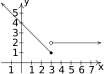
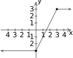
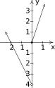
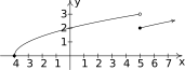
We said earlier in the section that it is not good enough to say local extrema exist where a function changes from increasing to decreasing or vice versa. As a previous exercise showed, we could have local extrema when a function is constant so now we need to examine some functions whose graphs do indeed change direction. Consider the functions graphed below. Notice that all four of them change direction at an open circle on the graph. Examine each for local extrema. What is the effect of placing the “dot” on the -axis above or below the open circle? What could you say if no function value were assigned to ?
Figure 1.174Function I
Figure 1.175Function II
Figure 1.176Function III
Figure 1.177Function IV
Answers
Domain:
-intercept:
-intercept:
No symmetry
Figure 1.178
Domain:
-intercept:
-intercept:
No symmetry
Figure 1.179
Domain:
-intercept: None
-intercept:
Even
Figure 1.180
Domain:
-intercepts: ,
-intercept:
Even
Figure 1.181
Domain:
-intercept: None
-intercept:
Even
Figure 1.182
Domain:
-intercept:
-intercept:
Odd
Figure 1.183
Domain:
-intercepts: , ,
-intercept:
No symmetry
Figure 1.184
Domain:
-intercept:
-intercept: None
No symmetry
Figure 1.185
Domain:
-intercept:
-intercept:
No symmetry
Figure 1.186
Domain:
-intercept:
-intercept:
No symmetry
Figure 1.187
Domain:
-intercept:
-intercept:
Odd
Figure 1.188
Domain:
-intercept: None
-intercept:
Even
Figure 1.189
Figure 1.190
Figure 1.191
Figure 1.192
Figure 1.193
Figure 1.194
Figure 1.195
Figure 1.196
Figure 1.197
odd
neither
even
even
even
neither
odd
odd
even
neither
neither
even
even and odd
odd
even
even
neither
odd
odd
even
even
, ,
, ,
neither
,
,
,
, ,
, ,
neither
,
none
,
none
No absolute maximum Absolute minimum Local minimum at Local maximum at Local minimum at Increasing on Decreasing on
No absolute maximum No absolute minimum Local maximum at Local minimum at Increasing on Decreasing on
Absolute maximum Absolute minimum Local maximum at No local minimum Increasing on Decreasing on
Absolute maximum Absolute minimum Local maximum Local minimum Increasing on Decreasing on
, so the Sasquatch is 2 feet tall at birth.
, so the Saquatch is 6 feet tall when she is 15 years old.
when and . This means the Sasquatch is 6 feet tall when she is 15 and 60 years old.
is constant on . This means the Sasquatch's height is constant (at 8 feet) for these years.
is decreasing on . This means the Sasquatch is getting shorter from the age of 45 to the age of 60. (Sasquatchteoporosis, perhaps?)
Figure 1.198The graph of .
Note that , but , so is neither even nor odd.
Adapted from Precalculus, 3rd corrected edition, by Carl Stitz and Jeff Zeager (stitz-zeager.com), licensed under CC BY-NC-SA 3.0. Changes were made: reformatted as an accessible XYZ web edition. License: CC-BY-NC-SA-3.0.
These eBooks are a prerelease and are not yet certified conformant with WCAG 2.1 AA or ADA Title II. Every page is built against an automated accessibility gate, and the published editions will meet ADA Title II requirements when they release in late September 2026. If something is unusable, please tell us.