In the previous section we used the newly defined function notation to make sense of expressions such as `' and `' for a given function . It would seem natural, then, that functions should have their own arithmetic which is consistent with the arithmetic of real numbers. The following definitions allow us to add, subtract, multiply and divide functions using the arithmetic we already know for real numbers.
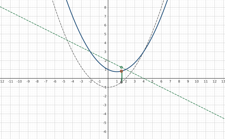
Interactive figure(f + g)(a) = f(a) + g(a): add the heights, one input at a timeDrag the Input a slider from -5 to 6.
XYZ Graph · viewer build 5edf91b
The two dashed curves are f(x) = x²/4 − 1 and g(x) = 2 − x/2; the solid curve is their sum f + g. At the input a set by the slider, the three marked heights are f(a), g(a) and (f + g)(a), and the two stacked vertical segments show the sum being assembled: the green segment is g(a) placed on top of the gray segment f(a), ending exactly at the solid curve. Slide a across the picture and the stacking is redone at every input, including places where one height is negative and the segments partly cancel, which is all function addition means.
Function Arithmetic
Suppose and are functions and is in both the domain of and the domain of .1
The sum of and , denoted , is the function defined by the formula
The difference of and , denoted , is the function defined by the formula
The product of and , denoted , is the function defined by the formula
The quotient of and , denoted , is the function defined by the formula
provided .
In other words, to add two functions, we add their outputs; to subtract two functions, we subtract their outputs, and so on. Note that while the formula looks suspiciously like some kind of distributive property, it is nothing of the sort; the addition on the left hand side of the equation is function addition, and we are using this equation to define the output of the new function as the sum of the real number outputs from and .
Please note the importance of finding the domain of a function before simplifying its expression. In number in Example 1.5.1 above, had we waited to find the domain of until after simplifying, we'd just have the formula to go by, and we would (incorrectly!) state the domain as , since the other troublesome number, , was canceled away.2
Next, we turn our attention to the difference quotient of a function.
We will revisit this concept in Section 2.1, but for now, we use it as a way to practice function notation and function arithmetic. For reasons which will become clear in Calculus, `simplifying' a difference quotient means rewriting it in a form where the `' in the definition of the difference quotient cancels from the denominator. Once that happens, we consider our work to be done.
As mentioned before, we will revisit difference quotients in Section 2.1 where we will explain them geometrically. For now, we want to move on to some classic applications of function arithmetic from Economics and for that, we need to think like an entrepreneur.4
Suppose you are a manufacturer making a certain product.5 Let be the production level, that is, the number of items produced in a given time period. It is customary to let denote the function which calculates the total cost of producing the items. The quantity , which represents the cost of producing no items, is called the fixed cost, and represents the amount of money required to begin production. Associated with the total cost is cost per item, or average cost, denoted and read `-bar' of . To compute , we take the total cost and divide by the number of items produced to get
On the retail end, we have the price
charged per item. To simplify the dialog and computations in this text, we assume that the number of items sold equals the number of items produced. From a retail perspective, it seems natural to think of the number of items sold, , as a function of the price charged, . After all, the retailer can easily adjust the price to sell more product. In the language of functions, would be the dependent variable and would be the independent variable or, using function notation, we have a function . While we will adopt this convention later in the text,6 we will hold with tradition at this point and consider the price as a function of the number of items sold, . That is, we regard as the independent variable and as the dependent variable and speak of the price-demand function, . Hence, returns the price charged per item when items are produced and sold. Our next function to consider is the revenue function, . The function computes the amount of money collected as a result of selling items. Since is the price charged per item, we have . Finally, the profit function, calculates how much money is earned after the costs are paid. That is, . We summarize all of these functions below.
Summary of Common Economic Functions
Suppose represents the quantity of items produced and sold.
The price-demand function calculates the price per item.
The revenue function calculates the total money collected by selling items at a price , .
The cost function calculates the cost to produce items. The value is called the fixed cost or start-up cost.
The average cost function calculates the cost per item when making items. Here, we necessarily assume .
The profit function calculates the money earned after costs are paid when items are produced and sold, .
It is high time for an example.
Exercises
In Exercises -, use the pair of functions and to find the following values if they exist.
and
and
and
and
and
and
and
and
and
and
In Exercises -, use the pair of functions and to find the domain of the indicated function then find and simplify an expression for it.
and
and
and
and
and
and
and
and
and
and
In Exercises -, find and simplify the difference quotient for the given function.
where
where
, where .
. HINT:
In Exercises -, denotes the cost to produce items and denotes the price-demand function in the given economic scenario. In each Exercise, do the following:
Find and interpret .
Find and interpret .
Find and interpret
Find and simplify .
Find and simplify .
Solve and interpret.
The cost, in dollars, to produce “I'd rather be a Sasquatch” T-Shirts is , and the price-demand function, in dollars per shirt, is , .
The cost, in dollars, to produce bottles of All-Natural Certified Free-Trade Organic Sasquatch Tonic is , and the price-demand function, in dollars per bottle, is , .
The cost, in cents, to produce cups of Mountain Thunder Lemonade at Junior's Lemonade Stand is , and the price-demand function, in cents per cup, is , .
The daily cost, in dollars, to produce Sasquatch Berry Pies , and the price-demand function, in dollars per pie, is , .
The monthly cost, in hundreds of dollars, to produce custom built electric scooters is , and the price-demand function, in hundreds of dollars per scooter, is , .
In Exercises -, let be the function defined by
and let be the function defined
. Compute the indicated value if it exists.
Answers
For and
For and
For and
For and
For and
For and
For and
For and
For and
is undefined.
For and
For and
Domain:
Domain:
Domain:
Domain:
For and
Domain:
Domain:
Domain:
Domain:
For and
Domain:
Domain:
Domain:
Domain:
For and
Domain:
Domain:
Domain:
Domain:
For and
Domain:
Domain:
Domain:
Domain:
For and
Domain:
Domain:
Domain:
Domain:
For and
Domain:
Domain:
Domain:
Domain:
For and
Domain:
Domain:
Domain:
Domain:
For and
Domain:
Domain:
Domain:
Domain:
For and
Domain:
Domain:
Domain:
Domain:
, so the fixed costs are .
, so when 10 shirts are produced, the cost per shirt is .
, so to sell shirts, set the price at per shirt.
,
,
when and . These are the `break even' points, so selling shirt or shirts will guarantee the revenue earned exactly recoups the cost of production.
, so the fixed costs are .
, so when 10 bottles of tonic are produced, the cost per bottle is .
, so to sell bottles of tonic, set the price at per bottle.
,
,
when and . These are the `break even' points, so selling bottles of tonic or bottles of tonic will guarantee the revenue earned exactly recoups the cost of production.
, so the fixed costs are ¢ or .
, so when 10 cups of lemonade are made, the cost per cup is ¢.
, so to sell cups of lemonade, set the price at ¢ per cup.
,
,
when and . These are the `break even' points, so selling cups of lemonade or cups of lemonade will guarantee the revenue earned exactly recoups the cost of production.
, so the daily fixed costs are .
, so when 10 pies are made, the cost per pie is .
, so to sell pies a day, set the price at per pie.
,
,
when and . These are the `break even' points, so selling pies or pies a day will guarantee the revenue earned exactly recoups the cost of production.
, so the monthly fixed costs are
hundred dollars, or .
, so when 10 scooters are made, the cost per scooter is hundred dollars, or .
, so to sell scooters a month, set the price at hundred dollars, or per scooter.
,
,
when and . These are the `break even' points, so selling scooters or scooters a month will guarantee the revenue earned exactly recoups the cost of production.
does not exist
does not exist
Adapted from Precalculus, 3rd corrected edition, by Carl Stitz and Jeff Zeager (stitz-zeager.com), licensed under CC BY-NC-SA 3.0. Changes were made: reformatted as an accessible XYZ web edition. License: CC-BY-NC-SA-3.0.
These eBooks are a prerelease and are not yet certified conformant with WCAG 2.1 AA or ADA Title II. Every page is built against an automated accessibility gate, and the published editions will meet ADA Title II requirements when they release in late September 2026. If something is unusable, please tell us.