
6.6 Quartiles
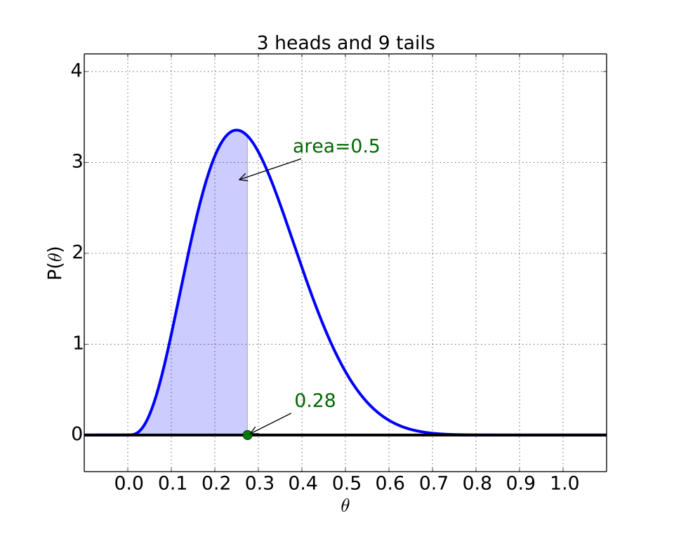
Given that we are dealing most often with continuous distributions, and thus need to look at areas under the curve from one point to another, it is useful to make a table for a distribution of these areas. Typically we look at the values of the parameter at which we have a given area under the curve from the minimum possible value of the parameter up to to that value. For example, we might be interested in the value of (i.e. how skewed the coin is) such that we have an area of 50% from 0 up to , shown in Figure 6.8. This point (called the median) represents the point where we would be just as confident (given our data) that the coin is more skewed than this as less skewed.
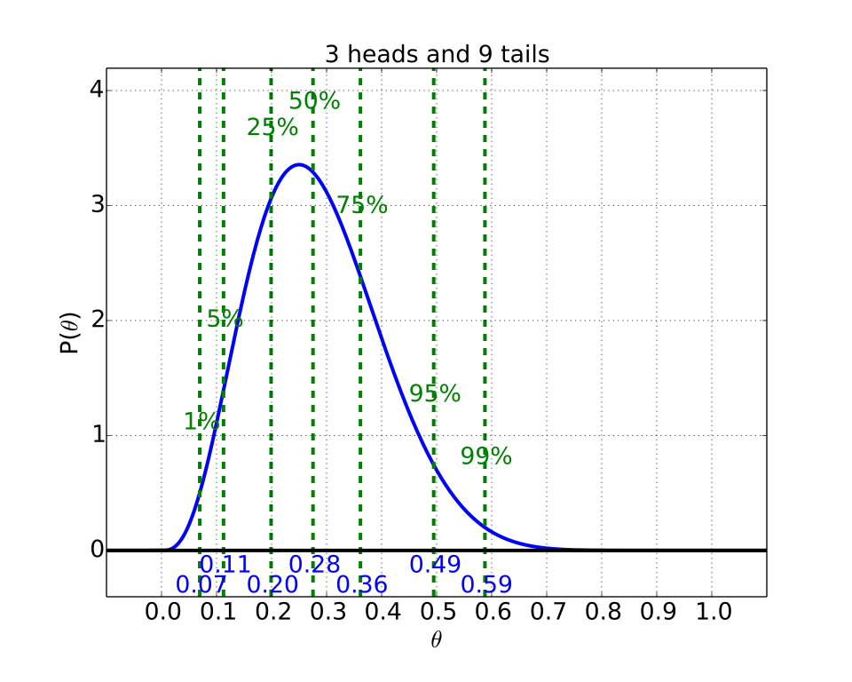
A table of these values for a distribution can be very useful. For example, consider the table and plot shown in Figure 6.9. Shown are the various points where the area under the curve up to those points is specified. For example, the area under the curve from up to is 5%. This means, given the data of 3 heads and 9 tails, there is a probability of the coin having less than , or an extreme skew towards tails.
Quartiles The term quartiles refers to the values of the parameter which result in an area of 25%, 50%, or 75%, or one, two, or three quarters of the area.
When we wish to refer to a non-quarter percentage, then we'll call it a percentile.
Percentiles The term percentile refers to the value of the parameter which result in a particulare area under the curve.
For example, we can say from Figure 6.9 that the 99% percentile is 0.59. Thus, it is extremely unlikely to have the coin skewed towards heads more than given the observation that we flipped 3 heads and 9 tails with this coin.
| Beta( heads=3, tails=9) | |
|---|---|
| Value | Area |
| 0.07 | 0.01 |
| 0.11 | 0.05 |
| 0.14 | 0.10 |
| 0.20 | 0.25 |
| 0.28 | 0.50 |
| 0.36 | 0.75 |
| 0.44 | 0.90 |
| 0.49 | 0.95 |
| 0.59 | 0.99 |
Adapted from Statistical Inference for Everyone, by Brian Blais (Bryant University), licensed under CC BY-SA 4.0 (dual-licensed under the GNU FDL 1.2 or later; this adaptation uses the CC BY-SA grant). Changes were made; this adaptation is distributed under the same license. License: CC-BY-SA-4.0.