Now we revisit the questions posed in Section 6.2 on page 121 about the bent coin, this time using the distribution found above, reproduced here in Figure 6.6.
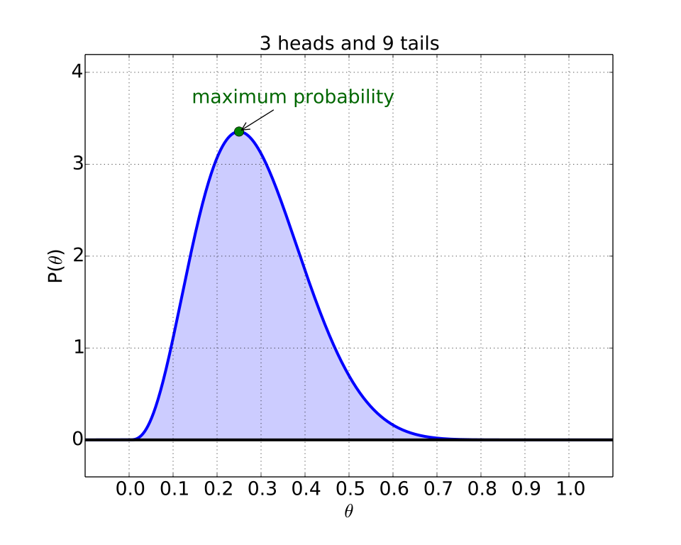
Figure 6.6. Posterior probability distribution for the values of the bent coin - the probability that the coin will land heads. The distribution is shown for data 3 heads and 9 tails, with a maximum at .
One answer to the first question can be accomplished by looking at the maximum of the posterior distribution, shown in Figure 6.6. By eye, it seems to have a maximum at . In fact one can demonstrate that this distribution has a maximum at
where in our example, a success is head, and an attempt is a flip. We take up this question of the best estimate of , given the posterior probability for , in more detail in Section 6.7.
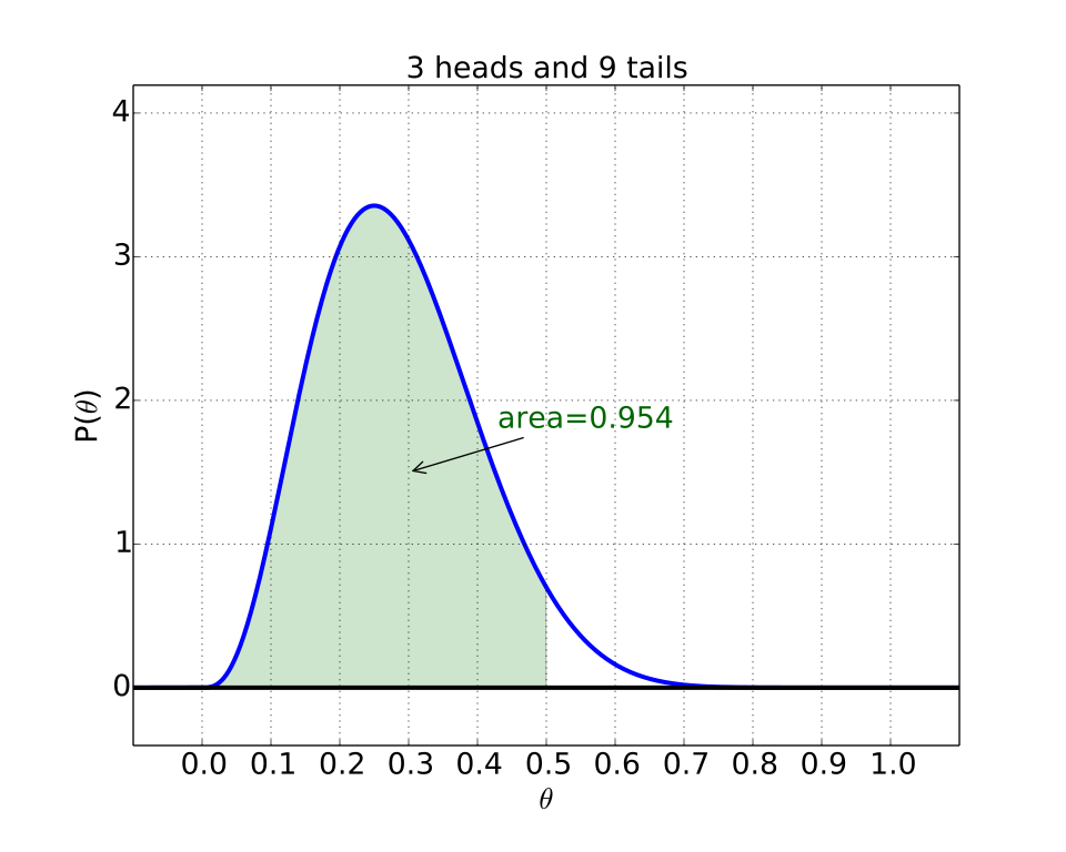
The answer to the second question can be done by looking at the area under the curve from , the “all heads” coin, to , the “fair” coin, as shown in Figure 6.7. This area represents the probability, given the data, that the coin is skewed towards heads or, in other words, how confident are we that this is an unfair coin. Given the value of we can say that this is “very likely” an unfair coin (see Table 1.1 on page 51).
Figure 6.7. Posterior probability distribution for the values of the bent coin - the probability that the coin will land heads. The distribution is shown for data 3 heads and 9 tails. The area under the curve from (the “all heads” coin) to (the “fair” coin) is 0.954.
Adapted from Statistical Inference for Everyone, by Brian Blais (Bryant University), licensed under CC BY-SA 4.0 (dual-licensed under the GNU FDL 1.2 or later; this adaptation uses the CC BY-SA grant). Changes were made; this adaptation is distributed under the same license. License: CC-BY-SA-4.0.
These eBooks are a prerelease and are not yet certified conformant with WCAG 2.1 AA or ADA Title II. Every page is built against an automated accessibility gate, and the published editions will meet ADA Title II requirements when they release in late September 2026. If something is unusable, please tell us.