
6.4 Moving Toward the Continuous
There is a practical problem that we face at this point, when we consider a generic bent coin. Perhaps it doesn't fit in one of the 11 models considered, falling somewhere in between, for example with . Ones' first thought might be to include one thousand coins or one million coins instead of the 11 we've considered so far, so we could have coin 132464, coin 132465, coin 132466, etc... Although this can be done, we run into two problems
- Because we are dealing with so many models, the probability associated with any single model gets very small - and gets smaller with the more models you consider
- We can't practically distinguish between models such as and (the last digit is different here)
In order to solve both of these problems mathematically, we introduce the concept of a continuous distribution. We start by labeling the model with a continuous number rather than an integer. In our present case it makes sense to label the model with the probability that the coin flips heads. We'll call this label , and it will have a value between 0 (heads are impossible) and 1 (heads are certain) and can take on any value in between. Because we now have an infinite number of labels, we have two consequences:
- We can't simply add up all the probabilities to get our value of to make everything add up to 1. Instead, we look at areas under the curve and make sure the entire area equals 1.
- Because, with distributions, areas under the curve (and not the values of the distribution itself) are the probabilities, we can only speak about ranges of values. For example, we can speak meaningfully about the probability of between 0.3 and 0.4 (i.e. ). When we write down something like we're not talking about a probability of a single label but rather the magnitude of the distribution at that label, .
We revisit Bayes' Recipe again, using the distributions. This time we also will look at pictures of the distributions as we progress.
![Function graph showing y = (x^h*(1-x)^t)/((h/(h+t))^h*(1-h/(h+t))^t) on x in [0, 1] with the region between the curve and the x-axis shaded and y = exp(-((x-h/(h+t))/0.005)^2) on x in [0, 1]. Adjustable parameters: Heads observed (h) = 3, Tails observed (t) = 9. Viewing window: x from -0.07 to 1.13, y from -0.13 to 1.07.](figures/xg-blais-ch06-bentcoin-posterior.svg)
- Specify the prior probabilities for the models being considered:
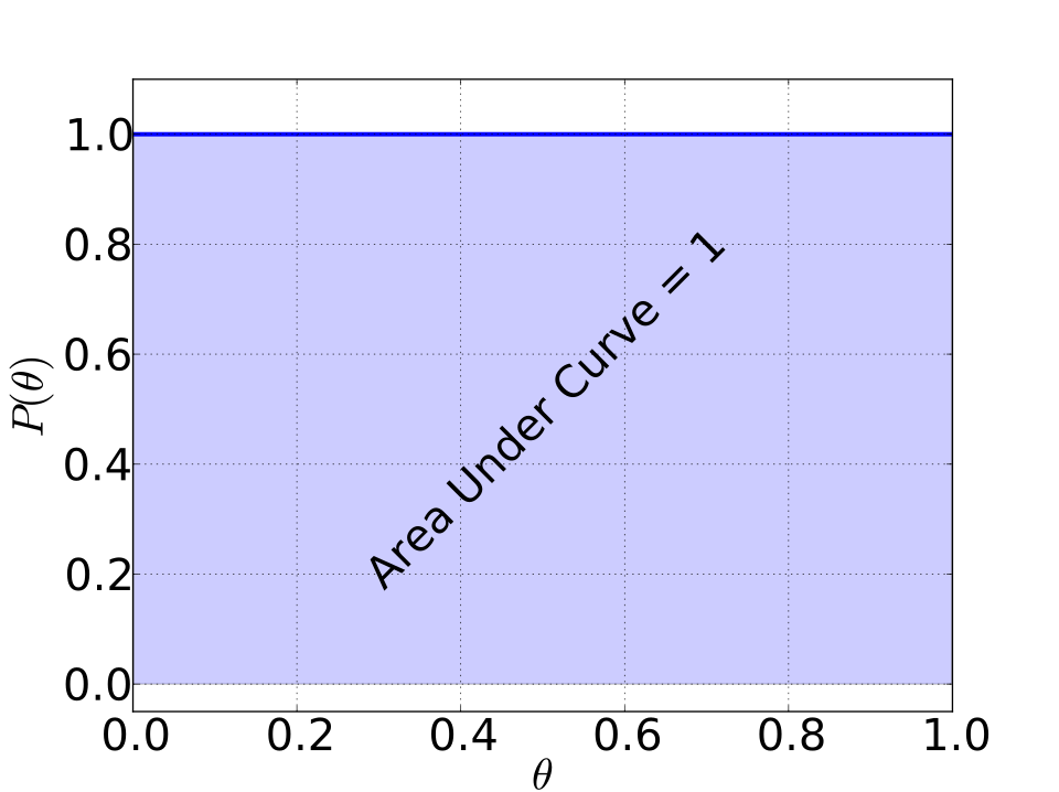
- Write the top of Bayes' Rule for all models being considered:
We can write one equation for all of the models labeled by at once as
- Put in the likelihood and prior values.
We use the binomial model, one equation for all models, remembering that for a model labeled by the probability for that coin flipping heads is . Thus we get the likelihood and prior values as
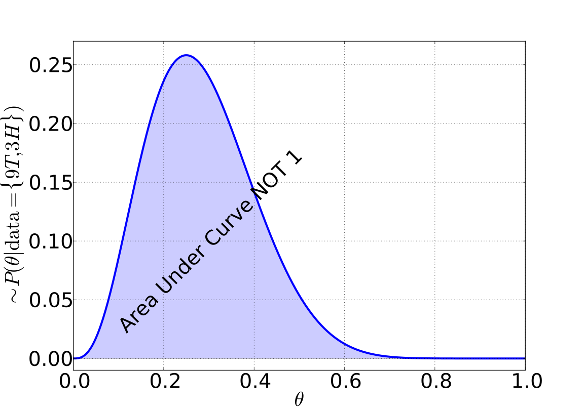
- Find the area under this curve, and call it .
- Divide each of the values of the curve by this are, , to get the final probabilities where the area under the curve is 1.
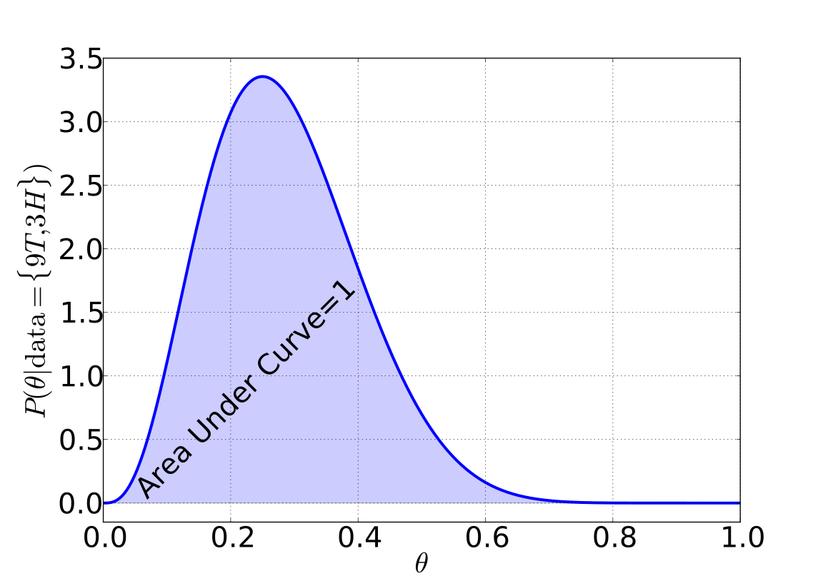
Usually these steps are done for you, for a specific data set, and you are given the final posterior distribution to use in answering any questions. However, for any particular case it is important to know what assumptions have been made in the choice of models and model parameters.
Adapted from Statistical Inference for Everyone, by Brian Blais (Bryant University), licensed under CC BY-SA 4.0 (dual-licensed under the GNU FDL 1.2 or later; this adaptation uses the CC BY-SA grant). Changes were made; this adaptation is distributed under the same license. License: CC-BY-SA-4.0.