
6.11 Computer Examples
from sie import *Beta Distribution Example
3 heads and 9 tails
Plot a beta distribution with 3 heads and 9 tails...
dist=beta(h=1,N=3)
distplot(dist,xlim=[0,1],show_quartiles=False)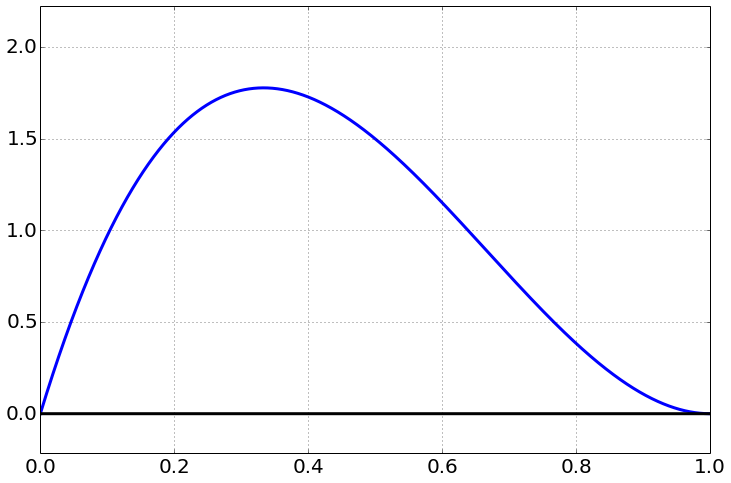
The median of this distribution...
dist.median()Show expected output
0.27527583248615201the 95
credible_interval(dist)Show expected output
(0.067585986488542985, 0.38572756813238962, 0.80587955031675662)1 heads and 3 tails
This should be about the same fraction as the previous example, but broader
dist=beta(h=1,N=4)
distplot(dist,xlim=[0,1])
Show expected output
<matplotlib.figure.Figure at 0x108768cd0>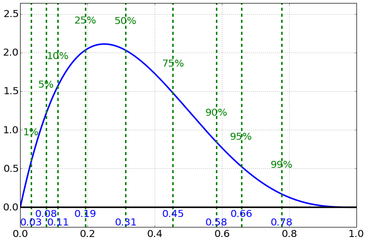
credible_interval(dist)Show expected output
(0.052744950526316919, 0.31381017045569742, 0.71641793611808946)Adapted from Statistical Inference for Everyone, by Brian Blais (Bryant University), licensed under CC BY-SA 4.0 (dual-licensed under the GNU FDL 1.2 or later; this adaptation uses the CC BY-SA grant). Changes were made; this adaptation is distributed under the same license. License: CC-BY-SA-4.0.