12.4 Simple Linear Regression

A linear regression is a straight line that describes how the values of a response variable $y$ change as the predictor variable $x$ changes. The equation of a line, relating $x$ to $y$ uses the slope-intercept form of a line, but with different letters than what you may be used to in a math class. We let $b sub 0$ represent the sample $y$ -intercept (the value of $y$ when $x equals 0$ ), $b sub 1$ the sample slope (rise over run), and $\hat{y}$ the predicted value of $y$ for a specific value of $x$ . The equation is written as $\hat{y} = b_{0} + b_{1} x$ .

Some textbooks and the TI calculators use the letter $a$ to represent the $y$ -intercept and $b$ to represent the slope, and the equation is written as $\hat{y} = a + b x$ . These letters are just symbols representing the placeholders for the numeric values for the $y$ -intercept and slope.

If we were to fit the best line that was closest to all the points on the scatterplot we would get what we call the “line of best fit,” also known as the “regression equation” or “least squares regression line.” Figure 12-9 is a scatterplot with just five points.

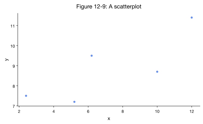
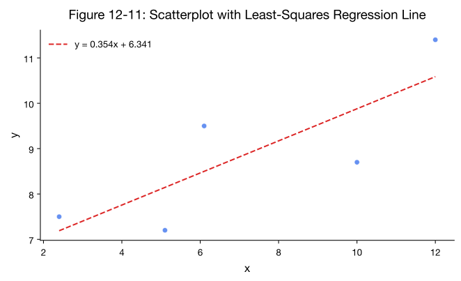
A scatterplot containing 5 points. — Figure 12-9: A scatterplot.

Figure 12-10 shows the least-squares regression line of $y$ on $x$ , which is the line that minimizes the squared vertical distance from all of the data. If we were to fit the line that best fits through the points, we would get the line pictured below.

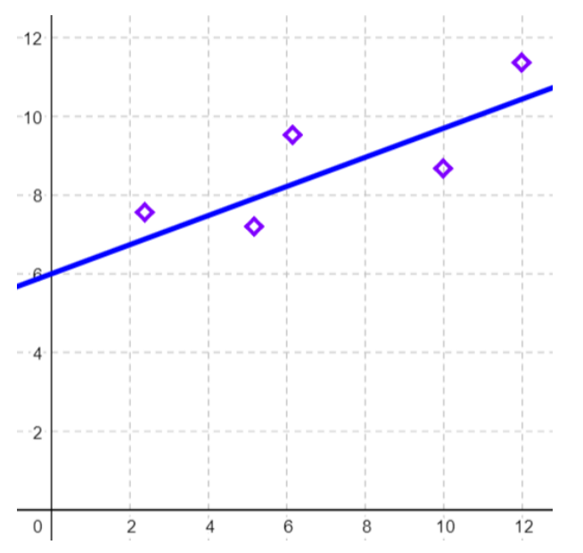
The scatterplot, containing an additional line that passes roughly an equal distance from each of the points. — Figure 12-10: Scatterplot with least-squares regression line.

What we want to look for is the minimum of the squared vertical distance between each point and the regression equation, called a residual. This is where the name of the least squares regression line comes from. Figure 12-11 shows the squared residuals.

Scatterplot with regression line and squared residuals. Residuals are represented by each point above the line being located at the top left corner of a square whose lower left corner rests on the line, and each point below the line being at the bottom left corner of a square whose upper left corner rests on the line. — Figure 12-11: Scatterplot with least-squares regression line and squared residuals.

To find the slope and $y$ -intercept for the equation of the least-squares regression line $\hat{y} = b_{0} + b_{1} x$ we use the following formulas: slope $= b_{1} = \frac{S S_{x y}}{S S_{x x}}$ , $y$ -intercept: $b_{0} = \bar{y} - b_{1} \bar{x}$ .

To compute the least squares regression line, you will need to first find the slope. Then substitute the slope into the following equation of the $y$ -intercept: $b_{0} = \bar{y} - b_{1} \bar{x}$ , where $\bar{x}$ = the sample mean of the $x$ ’s and $\bar{y}$ = the sample mean of the $y$ ’s.

Once we find the equation for the regression line, we can use it to estimate the response variable $y$ for a specific value of the predictor variable $x$ .

Note: we would only want to use the regression equation for prediction if we reject $H sub 0$ and find that there is a significant correlation between $x$ and $y$ . Alternatively, we could start with the regression equation and then test to see if the slope is significantly different from zero.

Example 1

Use the following data to find the line of best fit.

Hours Studied for Exam 20 16 20 18 17 16 15 17 15 16 15 17 16 17 14 Grade on Exam 89 72 93 84 81 75 70 82 69 83 80 83 81 84 76

Show solution

Start with finding the 2-Var Stats and sum of squares as shown in the steps for correlation.

$S S_{x x} = (n - 1) s_{x}^{2} = (15 - 1) {1.723783215}^{2} = 41.6$

$S S_{y y} = (n - 1) s_{y}^{2} = (15 - 1) {6.717425811}^{2} = 631.7333$

$S S_{x y} = \sum (x y) - n \cdot \bar{x} \cdot \bar{y} = 20087 - (15 \cdot 16.6 \cdot 80.133333) = 133.8$

Calculate the slope: $b_{1} = \frac{S S_{x y}}{S S_{x x}} = \frac{133.8}{41.6} = 3.216346$ .

Calculate the $y$ -intercept: $b_{0} = \bar{y} - b_{1} \cdot \bar{x} = 80.133333 - 3.216346 \cdot 16.6 = 26.742$ .

Put these numbers back into the regression equation and write your answer as: $\hat{y} = 26.742 + 3.216346 x$ .

Interpreting the $y$ -intercept coefficient: When $x equals 0$ , note that $y hat equals 26.742$ . This means that we would expect a failing midterm score of 26.742 for students who had studied zero hours.

Interpreting the slope coefficient: For each additional hour studied for the exam, we would expect an increase in the midterm grade of 3.2163 points.

In general, when interpreting the slope coefficient, for each additional 1 unit increase in $x$ , the predicted $\hat{y}$ value will change by $b sub 1$ units.

Adding the Regression Line to the Scatterplot

TI-84: Make a scatterplot using the directions from the previous section. Turn your STAT scatter plot on. Press [Y=] and clear any equations that are in the $y$ -editor. Into Y1, enter the least-squares regression equation manually as found above. Or, press the VARS key, go to option 5: Statistics, arrow over to EQ for equation, then choose the first option RegEQ. This will bring the equation over to the Y= menu without rounding error. Press [GRAPH]. You can press [TRACE] and use the arrow keys to scroll left or right. Pressing up or down on the arrow keys will change between tracing the scatterplot and the regression line. You can use the regression line to predict values of the response variable for a given value of the explanatory variable. While tracing the regression line type the value of the explanatory variable and press [ENTER]. For example, for $x equals 19$ the value of $y hat equals 87.8526$ .

TI-89: Make a scatterplot and find the regression line using the directions in the previous section. If you press [♦] then [F1] (Y=) you will notice the regression equation has been stored into y1 in the y-editor. Press [F2] Trace and use the left and right arrow keys to trace along the plot. Use the up and down arrow keys to toggle between the regression line and the scatterplot. You can use the regression line to predict values of the response variable for a given value of the explanatory variable. While tracing the regression line type the value of the explanatory variable and press [ENTER]. For example, for $x equals 19$ the value of $y equals 87.8526$ .

Adapted from Mostly Harmless Statistics by Rachel Webb (Portland State University), hosted on LibreTexts (stats.libretexts.org) and licensed under CC BY-SA 4.0. Changes were made. License: CC-BY-SA-4.0.