12.3 Hypothesis Test for a Correlation

One should perform a hypothesis test to determine if there is a statistically significant correlation between the independent and the dependent variables. The population correlation coefficient $\rho$ (this is the Greek letter rho, which sounds like “row” and is not a $p$ ) is the correlation among all possible pairs of data values $(x, y)$ taken from a population.

We will only be using the two-tailed test for a population correlation coefficient $\rho$ . The hypotheses are:

$H_{0}: \rho = 0$
$H_{1}: \rho \neq 0$

The null-hypothesis of a two-tailed test states that there is no correlation (there is not a linear relation) between $x$ and $y$ . The alternative-hypothesis states that there is a significant correlation (there is a linear relation) between $x$ and $y$ .

The t-test is a statistical test for the correlation coefficient. It can be used when $x$ and $y$ are linearly related, the variables are random variables, and when the population of the variable $y$ is normally distributed.

The formula for the t-test statistic is $t = r \sqrt{\left( \dfrac{n-2}{1-r^{2}} \right)}$ .

Use the t-distribution with degrees of freedom equal to $df = n - 2$ .

Note the $df = n - 2$ since we have two variables, $x$ and $y$ .

Example 1

Test to see if the correlation for hours studied on the exam and grade on the exam is statistically significant. Use $\alpha$ = 0.05.

Hours Studied for Exam 20 16 20 18 17 16 15 17 15 16 15 17 16 17 14 Grade on Exam 89 72 93 84 81 75 70 82 69 83 80 83 81 84 76

Show solution

The hypotheses are:

$H_{0}: \rho = 0$
$H_{1}: \rho \neq 0$

Find the critical value using $df = n -2 = 13$ for a two-tailed test $\alpha= 0.05$ inverse t-function to get the critical values $\pm 2.160$ . Draw the sampling distribution and label the critical values as shown in Figure 12-5.

Figure 12-5: Sampling distribution of t-function with critical values labeled.

Next, find the test statistic $t = r \sqrt{\left( \frac{n-2}{1-r^{2}} \right)} = 0.8254 \sqrt{\left( \frac{13}{1 - 0.8254^{2}} \right)} = 5.271$ , which is greater than 2.160 and in the rejection region.

Summary: At the 5% significance level, there is enough evidence to support the claim that there is a statistically significant linear relationship (correlation) between the number of hours studied for an exam and exam scores.

The p-value method could also be used to find the same decision. We will use technology shortcuts for the p-value method. The p-value = $2 \cdot \text{P}(t \geq 5.271 | H_{0} \text{ is true}) = 0.000151$ , which is less than $\alpha$ = 0.05; therefore we reject $H_{0}$ .

Alternatively, we could test to see if the slope was equal to zero. If the slope is zero then the correlation will also be zero. The setup of a test is a little different, but we get the same results. Most software packages report the test statistic and p-value for a slope. This test is introduced in the next section.

TI-84: Enter the data in L₁ and L₂. Press the [STAT] key, arrow over to the [TESTS] menu, arrow down to the option [LinRegTTest] and press the [ENTER] key. The default is Xlist: L₁, Ylist: L₁, Freq:1, $\beta$ and $\rho: \neq 0$ . Arrow down to Calculate and press the [ENTER] key. The calculator returns the t-test statistic, p-value and the correlation coefficient = $r$ . Note the p-value = 0.0001513, is less than $\alpha$ = 0.05; therefore reject $H_{0}$ , as there is a significant correlation.

TI-89: Enter the data in List1 and List2. In the Stats/List Editor select F6 for the Tests menu. Use cursor keys to select A:LinRegTTest and press [Enter]. In the “X List” space type in the name of your list with the $x$ variable without space, for our example “list1” or use [2nd] [Var-Link] and highlight list1. In the “Y List” space type in the name of your list with the $y$ variable without space, for our example “list2” or use [2nd] [Var-Link] and highlight list2. Under the “Alternate Hyp” menu select the $\beta$ and $\rho: \neq 0$ option, which is the same as the question’s alternative hypothesis statement, then press the [ENTER] key, arrow down to [Calculate] and press the [ENTER] key. The calculator returns the t-test statistic, p-value, and the correlation = $r$ .

Excel: Type the data into two columns in Excel. Select the Data tab, then Data Analysis, then choose Regression and select OK.

Be careful here. The second column is the $y$ range, and the first column is the $x$ range. Only check the Labels box if you highlight the labels in the input range. The output range is one cell reference where you want the output to start, and then select OK.

Figure 12-6 shows the regression output.

Figure 12-6: Excel-generated regression output.

When you reject $H_{0}$ , the slope is significantly different from zero. This means there is a significant relationship (correlation) between $x$ and $y$ , and you can then find a regression line to use for prediction which we explore in the next section, called Simple Linear Regression.

Correlation is Not Causation

Just because two variables are significantly correlated does not imply a cause and effect relationship. There are several relationships that are possible. It could be that $x$ causes $y$ to change. You can actually swap $x$ and $y$ in the fields and get the same $r$ value and $y$ could be causing $x$ to change. There could be other variables that are affecting the two variables of interest. For instance, you can usually show a high correlation between ice cream sales and home burglaries. Selling more ice cream does not “cause” burglars to rob homes. More home burglaries do not cause more ice cream sales. We would probably notice that the temperature outside may be causing both ice cream sales to increase and more people to leave their windows open. This third variable is called a lurking variable and causes both $x$ and $y$ to change, making it look like the relationship is just between $x$ and $y$ .

There are also highly correlated variables that seemingly have nothing to do with one another. These seemingly unrelated variables are called spurious correlations.

The following website has some examples of spurious correlations (a slight caution that the author has some gloomy examples): http://www.tylervigen.com/spurious-correlations. Figure 12-7 is one of their examples:

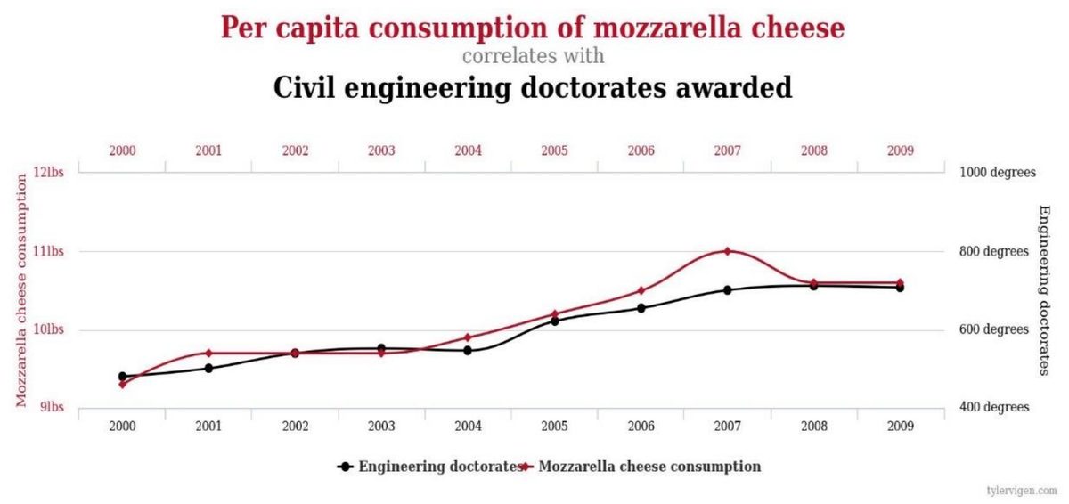
Chart from tylervigen.com, showing correlation from 2000 to 2009 between per-capita mozzerella cheese consumption number of civil engineering doctorates awarded. — Figure 12-7: Example of spurious correlations. (6/25/2020) Retrieved from http://tylervigen.com/view_correlation?id=28726.

If we were to take out each pair of measurements by year from the time-series plot in Figure 12-7, we would get the following data.

Year	Engineering Doctorates	Mozzarella Cheese Consumption
2000	480	9.3
2001	501	9.7
2002	540	9.7
2003	552	9.7
2004	547	9.9
2005	622	10.2
2006	655	10.5
2007	701	11
2008	712	10.6
2009	708	10.6

Using Excel to find a scatterplot and compute a correlation coefficient, we get the scatterplot shown in Figure 12-8 and a correlation of $r = 0.9586$ .

Excel-generated scatterplot of the spurious correlation example, with mozzarella cheese consumption on the x-axis and engineering doctorates on the y-axis. — Figure 12-8: Scatterplot for spurious correlation example.

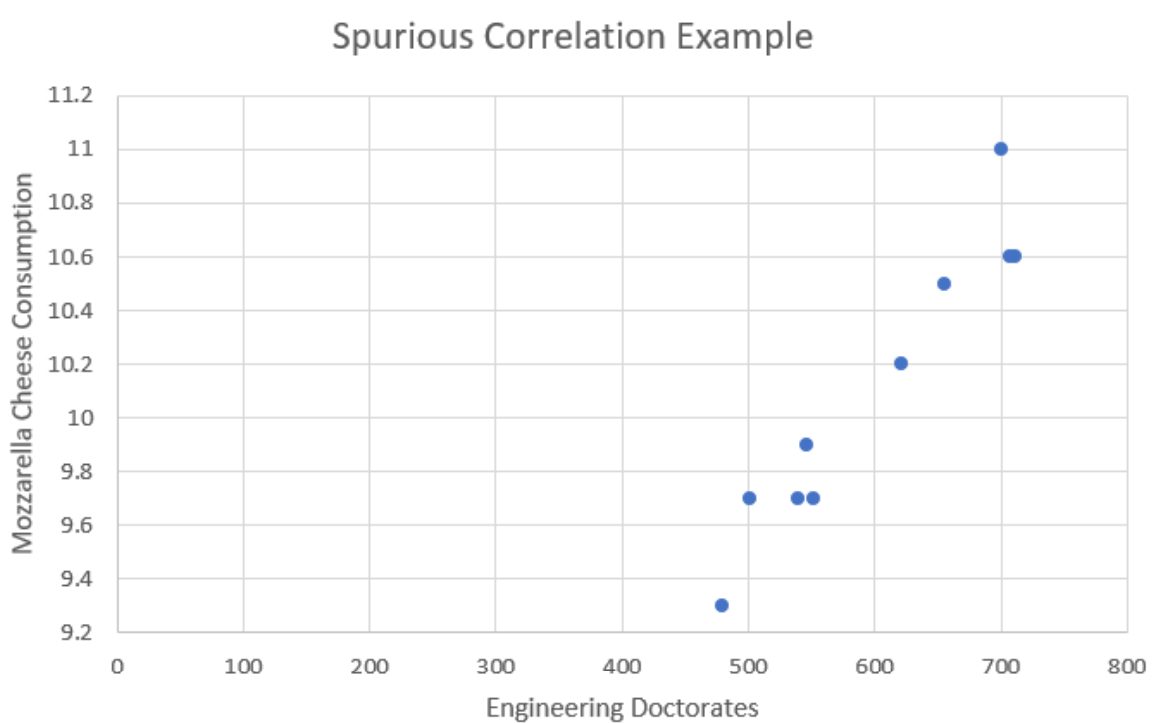
With $r = 0.9586$ , there is strong correlation between the number of engineering doctorate degrees earned and mozzarella cheese consumption over time, but earning your doctorate degree does not cause one to go eat more cheese. Nor does eating more cheese cause people to earn a doctorate degree. Most likely these items are both increasing over time and therefore show a spurious correlation to one another.

When two variables are correlated, it does not imply that one variable causes the other variable to change.

“Correlation is causation” is an incorrect assumption that because something correlates, there is a causal relationship. Causality is the area of statistics that is most commonly misused, and misinterpreted, by people. Media, advertising, politicians and lobby groups often leap upon a perceived correlation and use it to “prove” their own agenda. They fail to understand that, just because results show a correlation, there is no proof of an underlying causality. Many people assume that because a poll, or a statistic, contains many numbers, it must be scientific, and therefore correct. The human brain is built to try and subconsciously establish links between many pieces of information at once. The brain often tries to construct patterns from randomness, and may jump to conclusions, and assume that a cause and effect relationship exists. Relationships may be accidental or due to other unmeasured variables. Overcoming this tendency to jump to a cause and effect relationship is part of academic training for students and in most fields, from statistics to the arts.

Summary

When looking at correlations, start with a scatterplot to see if there is a linear relationship prior to finding a correlation coefficient. If there is a linear relationship in the scatterplot, then we can find the correlation coefficient to tell the strength and direction of the relationship. Clusters of dots forming a linear uphill pattern from left to right will have a positive correlation. The closer the dots in the scatterplot are to a straight line, the closer $r$ will be to $1$ . If the cluster of dots in the scatterplots go downhill from left to right in linear pattern, then there is a negative relationship. The closer those dots in the scatterplot are to a straight line going downhill, the closer $r$ will be to $-1$ . Use a t-test to see if the correlation is statistically significant. As sample sizes get larger, smaller values of $r$ become statistically significant. Be careful with outliers, which can heavily influence correlations. Most importantly, correlation is not causation. When $x$ and $y$ are significantly correlated, this does not mean that $x$ causes $y$ to change.

Adapted from Mostly Harmless Statistics by Rachel Webb (Portland State University, https://mostlyharmlessstat.wixsite.com/webpage), © Rachel Webb, licensed under CC BY-SA 4.0. Changes were made. License: CC-BY-SA-4.0.