
Login
📚 Mostly Harmless Statistics
Chapters ▾

9 Hypothesis Tests and Confidence Intervals for Two Populations

9.01: Two Sample Mean T-Test for Dependent Groups

Dependent samples or matched pairs, occur when the subjects are paired up, or matched in some way. Most often, this model is characterized by selection of a random sample where each member is observed under two different conditions, before/after some experiment, or subjects that are similar (matched) to each other are studied under two different conditions.

There are 3 types of hypothesis tests for comparing two dependent population means µ1 and µ2, where, µD is the expected difference of the matched pairs.
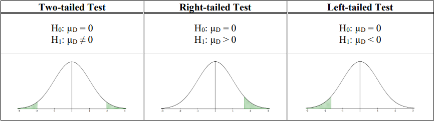
clipboard_e22a5f74fe6513fb63eecca19ef728c65.png
Figure 9-1

Note: If each pair were equal to one another then the mean of the differences would be zero. We could also use this model to test with a magnitude of a difference, but we rarely cover that scenario, therefore we are usually test against the difference of zero.

The t-test for dependent samples is a statistical test for comparing the means from two dependent populations (or the difference between the means from two populations). The t-test is used when the differences are normally distributed. The samples also must be dependent.

The formula for the t-test statistic is: \(t=\frac{\bar{D}-\mu_{D}}{\left(\frac{S_{D}}{\sqrt{n}}\right)}\).

Where the t-distribution with degrees of freedom, df = n – 1

Note we will usually only use the case where µD equals zero.

The subscript “D” denotes the difference between population one and two. It is important to compute D = x1 – x2 for each pair of observations. However, this makes setting up the hypotheses more challenging for one-tailed tests.

If we were looking for an increase in test scores from before to after, then we would expect the after score to be larger. When we take a smaller number minus a larger number then the difference would be negative. If we put the before group first and the after group second then we would need a left-tailed test μD < 0 to test the “increase” in test scores. This is opposite of the sign we associate for “increase.” If we swap the order and use the after group first, then the before group would have a larger number minus a smaller number which would be positive and we would do a right-tailed test μD > 0.

Always subtract in the same order the data is presented in the question. An easier way to decide on the one-tailed test is to write down the two labels and then put a less than () symbol between them depending on the question. For example, if the research statement is a weight loss program significantly decreases the average weight, the sign of the test would change depending on which group came first. If we subtract before weight – after weight, then we would want to have before > after and use μD > 0. If we have the after weight as the first measurement then we would subtract the after weight – before weight and want after < before and use μD < 0. If you keep your labels in the same order as they appear in the question, compare them and carry this sign down to the alternative hypothesis.

The traditional method (or critical value method), the p-value method, and the confidence interval method are performed with steps that are identical to those when performing hypothesis tests for one population.

A dietician is testing to see if a new diet program reduces the average weight. They randomly sample 35 patients and measure them before they start the program and then weigh them again after 2 months on the program. What are the correct hypotheses?

Solution

Let x1 = weight before a weight-loss program and x2 = weight after the weight-loss program. We want to test if, on average, participants lose weight. Therefore, the difference D = x1 – x2. This gives D = before weight – after weight, thus if on average people do lose weight, then in general the before > after and the D’s are positive. How we define our differences determines that this example is a right-tailed test (carry the > sign down to the alternative hypothesis) and the correct hypotheses are:

H0: µD = 0

H1: µD > 0

If we were to do the same problem but reverse the order and take D = after weight – before weight the correct alternative hypothesis is H1: µD < 0 since after weight < before weight. Just be consistent throughout your problem, and never switch the order of the groups in a problem.

P-Value Method Example

In an effort to increase production of an automobile part, the factory manager decides to play music in the manufacturing area. Eight workers are selected, and the number of items each produced for a specific day is recorded. After one week of music, the same workers are monitored again. The data are given in the table. At \(\alpha\) = 0.05, can the manager conclude that the music has increased production? Assume production is normally distributed. Use the p-value method.

Worker 1 2 3 4 5 6 7 8 Before 6 8 10 9 5 12 9 7 After 10 12 9 12 8 13 8 10
Solution

Assumptions: We are comparing production rates before and after music is played in the manufacturing area. We are given that the production rates are normally distributed. Because these are consecutive times from the same population, they are dependent samples, so we must use the t-test for matched pairs.

Let population 1 be the number of items before the music, and population 2 be after. The claim is that music increases production so before production < after production. Carry this same sign to the alternative hypothesis.

The correct hypotheses are: H0: µD = 0; H1: µD < 0, this is a left-tailed test.

In order to compute the t-test statistic, we must first compute the differences between each of the matched pairs.

Before (x1) 6 8 10 9 5 12 9 7
After (x2) 10 12 9 12 8 13 8 10
D = x1-x2 –4 –4 1 –3 –3 –1 1 –3

Using the 1-var stats on the differences in your calculator, we compute \(\bar{D}=\bar{x}=-2\), sD = sx = 2.0702, n = 8.

The test statistic is: \(\t=\frac{\bar{D}-\mu_{D}}{\left(\frac{s_{D}}{\sqrt{n}}\right)}=\frac{-2-0}{\left(\frac{2.0702}{\sqrt{8}}\right)}=-2.7325\).

The p-value for a two-tailed t-test with degrees of freedom = n – 1 = 7, is found by finding the area to the left of the test statistic –2.7325 using technology.

Decision: Since the p-value = 0.0146 is less than \(\alpha\) = 0.05, we reject H0.

Summary: At the 5% level of significance, there is enough evidence to support the claim that the mean production rate increases when music is played in the manufacturing area.

TI-84: Find the differences between the sample pairs (you can subtract two lists to do this). Press the [STAT] key and then the [EDIT] function, enter the difference column into list one. Press the [STAT] key, arrow over to the [TESTS] menu. Arrow down to the option [2:T -Test] and press the [ENTER]. Arrow over to the [Data] menu and press the [ENTER] key. Then type in the hypothesized mean as 0, List: L3, leave Freq:1 alone, arrow over to the \(\neq\), <, >, sign that is the same in the problem’s alternative hypothesis statement then press the [ENTER] key, arrow down to [Calculate] and press the [ENTER] key. The calculator returns the t-test statistic, the p-value, mean of the differences \(\bar{D}=\bar{x}\) and standard deviation of the differences sD = sx.

clipboard_ef43146b8f6de77736508a1fc6e915c15.png

TI-89: Find the differences between the sample pairs (you can subtract two lists to do this). Go to the [Apps] Stat/List Editor, enter the two data sets in lists 1 and 2. Move the cursor so that it is highlighted on the header of list3. Press [2nd] Var-Link and move down to list1 and press [Enter]. This brings the name list1 back to the list3 at the bottom, select the minus [-] key, then select [2nd] Var-link and this time highlight list2 and press [Enter]. You should now see list1-list2 at the bottom of the window. Press [Enter] then the differences will be stored in list3. Press [2nd] then F6 [Tests], select 2: T-Test. Select the [Data] menu. Then type in the hypothesized mean as 0, List: list1, Freq:1, arrow over to the \(\neq\), <, >, and select the sign that is the same in the problem’s alternative hypothesis, press the [ENTER] key to calculate. The calculator returns the t-test statistic, p-value, \(\bar{D}=\bar{x}\) and sD = sx.

clipboard_e80e009a4856da4f292f53a32b2554d95.png

clipboard_e4a4e262047f05122357d8b92d294dc2e.png

Excel: Start by entering the data in two columns in the same order that they appear in the problem. Then select Data > Data Analysis > t-test: Paired Two Sample for Means, then select OK.

Select the Before data (including the label) into the Variable 1 Range, and the After data (including the label) in the Variable 2 Range. Type in zero for the Hypothesized Mean Difference box. Select the box for Labels (do not select this if you do not have labels in the variable range selected). Change alpha to fit the problem. You can leave the default to open in a new worksheet or change output range to be one cell where you want the top left of the output table to start (make sure this cell does not overlap any existing data). Then select OK. See below for example.

clipboard_e6048d8250da8f0d0918357e77c4b454c.png

You get the following output:

clipboard_e71d370628fb1e563b44f30ae06af00c6.png

One nice feature in Excel is that you get the p-value and the critical value in the output. The critical value can be taken from the Excel output; however, Excel never gives negative critical values. Since we are doing a left-tailed test we will need to use the t-score = -1.8946.

If we were to draw and shade the critical region for the sampling distribution, it would look like Figure 9 -2.

clipboard_e46e4f3d152fea1d251982df8dfd9c7a0.png
Figure 9-2

The decision is made by comparing the test statistic t = -2.7325 with the critical value tα = -1.8946.

Since the test statistic is in the shaded critical region, we would reject H0.

At the 5% level of significance, there is enough evidence to support the claim that the mean production rate increases when music is played in the manufacturing area.

The decision and summary should not change from using the p-value method.

Confidence Interval Method

A (1 – \(\alpha\))*100% confidence interval for the difference between two population means with matched pairs: μD = mean of the differences.

\(\bar{D}-t_{\frac{\alpha}{2}}\left(\frac{s_{D}}{\sqrt{n}}\right)<\mu_{D}<\bar{D}+t_{\alpha / 2}\left(\frac{s_{D}}{\sqrt{n}}\right)\]

Or more compactly as \(\bar{D} \pm t_{\alpha / 2}\left(\frac{s_{D}}{\sqrt{n}}\right)\)

Where the t-distribution has degrees of freedom, df = n – 1, where n is the number of pairs.

Hands-On Cafe records the number of online orders for eight randomly selected locations for two consecutive days. Assume the number of online orders is normally distributed. Find the 95% confidence interval for the mean difference. Is there evidence of a difference in mean number of orders for the two days?

Location 1 2 3 4 5 6 7 8 Thursday 67 65 68 68 68 70 69 70 Friday 68 70 69 71 72 69 70 70
Solution

First set up the hypotheses. We are testing to see if Thursday \(\neq\) Friday orders. The hypotheses would be:

H0: µD = 0

H1: µD ≠ 0

Next, compute the \(\frac{t_

ParseError: invalid DekiScript (click for details)
Callstack:
    at (Bookshelves/Introductory_Statistics/Mostly_Harmless_Statistics_(Webb)/09:_Hypothesis_Tests_and_Confidence_Intervals_for_Two_Populations/9.01:_Two_Sample_Mean_T-Test_for_Dependent_Groups), /content/body/section[5]/div/table/div/p[4]/span, line 1, column 1
\) critical value for a 95% confidence interval and df = 7. Use the t-distribution with technology using confidence level 95%, lower tail area of \(\alpha\)/2 = 0.025 to get t\(\alpha\)/2 = t0.025 = ±2.36462. Compute the differences of Thursday – Friday for each pair.
Thursday 67 65 68 68 68 70 69 70
Friday 68 70 69 71 72 69 70 70
D –1 –5 –1 –3 –4 1 –1 0

Use technology to compute the mean, standard deviation and sample size.

Note if you use a TI calculator then \(\bar{D}=\bar{x}\) and sD = sx.

Find the interval estimate: \(\bar{D} \pm t_{\frac{\alpha}{2}}\left(\frac{s_{D}}{\sqrt{n}}\right)\)

\(\begin{aligned}
&\Rightarrow-1.75 \pm 2.36462\left(\frac{2.05287}{\sqrt{8}}\right) \\
&\Rightarrow-1.75 \pm 1.7162 .
\end{aligned}\)

Write the answer using standard notation –3.4662 < μD < –0.0335 or interval notation (–3.4662, –0.0338).

For an interpretation of the interval, if we were to use the same sampling techniques, approximately 95 out of 100 times the confidence interval (–3.4662, –0.0338) would contain the population mean difference in the number of orders between Thursday and Friday.

Since both endpoints are negative, we can be 95% confident that the population mean number of orders for Thursday is between 3.4662 and 0.0338 orders lower than Friday.

Excel: Type in both samples in two adjacent columns, and then subtract each pair in a third column and label the column Difference.

Thursday Friday Difference
67 68 =A2-B2
65 70 =A3-B3
68 69 =A4-B4
68 71 =A5-B5
68 72 =A6-B6
70 69 =A7-B7
69 70 =A8-B8
70 70 =A9-B9

Select Data > Data Analysis > Descriptive Statistics and click OK.

clipboard_ec1f263277d0b3135a58e2f1a8264cd8c.png

Select the Difference column for the input range including the label, then check the box next to Labels in first row (do not select this box if you did not highlight a label in the input range). Use the default new worksheet or select a single cell for the Output Range where you want your top left-hand corner of the table to start. Check the boxes Summary Statistics and Confidence Level for Mean. Change the confidence level to fit the question, and then select OK.

clipboard_e7b30dee2d19913ac74c852b89802ea7b.png

You get the following output:

clipboard_e756deaded61ca3ac563dcc22418919fd.png

The confidence interval is the mean ± margin of error. In two different cells subtract and then add the margin of error from the mean to get the confidence interval limits and then put your answer in interval notation (–3.4662, – 0.0338).

TI-84: First, find the differences between the samples. Then on the TI-83 press the [STAT] key, arrow over to the [TESTS] menu, arrow down to the [8:TInterval] option and press the [ENTER] key. Arrow over to the [Data] menu and press the [ENTER] key. The defaults are List: L1, Freq:1. If this is set with a different list, arrow down and use [2nd] [1] to get L1. Then type in the confidence level. Arrow down to [Calculate] and press the [ENTER] key. The calculator returns the confidence interval, \(\bar{D}=\bar{x}\) and sD = sx.

TI-89: First, find the differences between the samples. Go to the [Apps] Stat/List Editor, then enter the differences into list 1. Press [2nd] then F7 [Ints], then select 2: T-Interval. Select the [Data] menu. Enter in List: list1, Freq:1. Then type in the confidence level. Press the [ENTER] key to calculate. The calculator returns the confidence interval, \(\bar{D}=\bar{x}\) and sD = sx.

9.02: Two Independent Groups

This section will look at how to analyze a difference in the mean for two independent samples. As with all other hypothesis tests and confidence intervals, the process is the same, though the formulas and assumptions are different.

The symbol used for the population mean has been \(μ\) up to this point. In order to use formulas that compare the means from two populations, we use subscripts to show which population statistic or parameter we are referencing.

Parameters

Statistics

You do not need to use the subscripts 1 and 2. You can use a letter or symbol that helps you differentiate between the two groups. For instance, if you have two manufacturers labeled A and B, you may want to use µA and µB.

When setting up the null hypothesis we are testing if there is a difference in the two means equal to some known difference. H0: µ1 – µ2 = (µ1 – µ2)0. We will focus on the case where (µ1 – µ2)0 = 0, which says that, tentatively, we assume that there is no difference in population means H0: µ1 – µ2 = 0. If we were to subtract μ2 from both sides of the equation µ1 – µ2 = 0 we would get µ1 = µ2. For instance, if the average age for group one was 25 and the average age for group two was also 25, then the difference between the two means would be 25 – 25 = 0.

There are three ways to set up the hypotheses for comparing two independent population means µ1 and µ2.

clipboard_e8fb415dfc15b6fa8ee7b8f0e1cd0eaab.png

Figure 9-3

For a one-tailed test, one could alternatively write the null hypotheses as:

Right-tailed test Left-tailed test

H0: µ1 ≤ µ2 H0: µ1 ≥ µ2

H1: µ1 > µ2 H1: µ1 < µ2

This text mostly will use an = sign in the null hypothesis.

Most of the time the groups are numbered from the order in which their statistics or data appear in the problem. To keep the correct sign of the test, make sure you do not switch the order of the groups.

For instance, if we were comparing the mean SAT score between high school juniors and seniors and our hypothesis is that the mean for seniors is higher we could set up the alternative hypotheses as either µj < µs if we had the juniors be group 1 and µj > µs if we had the seniors be group 1. This change would switch the sign of both the test statistic and the critical value.

When performing a one-tailed test the sign of the test statistic and critical value will match most of the time. For example, if your test statistic came out to be z = –1.567 and your critical value was z = 1.645 you most likely have the incorrect order in your hypotheses.

When you are making a conjecture about a population mean, we have two different situations, depending on if we know that population standard deviation, or not, called the z-test and t-test, respectively. Use Figure 9-4 to help decide when to use the z-test and t-test.

clipboard_eab247afc8017175197885a2b75348545.png

Figure 9-4

Note that you should never use the value of σx on your calculator since you would rarely ever have an entire population of raw data to input into a calculator. The problem may give you raw data, but σ or σ2 would be stated in the problem and you should be using a z-test, otherwise use the t-test with the sample standard deviation sx. Usually, σ is known from a previous year or similar study.

In either case if the sample sizes are below 30 we need to check that the population is approximately normally distributed for the Central Limit Theorem to hold. We can do this with a normal probability plot. Most examples that we deal with just assume the population is normally distributed, but in practice, you should always check these assumptions.

9.3.1 Two Sample Mean Z-Test & Confidence Interval

The two-sample z-test is a statistical test for comparing the means from two independent populations with σ1 and σ2 stated in the problem and using the formula for the test statistic

\(z=\frac{\left(\bar{x}_{1}-\bar{x}_{2}\right)-\left(\mu_{1}-\mu_{2}\right)}{\sqrt{\left(\frac{\sigma_{1}^{2}}{n_{1}}+\frac{\sigma_{2}^{2}}{n_{2}}\right)}}\)

Note that µ1 – µ2 is the hypothesized difference found in the null hypothesis and is usually zero.

The traditional method (or critical value method), the p-value method, and the confidence interval method are performed with steps that are identical to those when performing hypothesis tests for one population. We will show an example of a two-sample z-test, but seldom in practice will we perform this type of test since we rarely have access to a population standard deviation.

A university adviser wants to see whether there is a significant difference in ages of full-time students and part-time students. They select a random sample of 50 students from each group. The ages are shown below. At \(\alpha\) = 0.05, decide if there is enough evidence to support the claim that there is a difference in the ages of the two groups. Assume the population standard deviation for full-time students is 3.68 years old and for part-time students is 4.7 years old. Use the p-value method.

Full-time students

22 25 27 23 26 28 26 24 25 20 19 18 30 26 18 18 19 32 23 19 18 22 26 19 19 21 23 18 20 18 22 18 20 19 23 26 24 27 26 18 22 21 19 21 21 19 18 29 19 22

Part-time students

18 20 19 18 22 25 24 35 23 18
24 26 30 22 22 22 21 18 20 19
19 32 29 23 21 19 36 27 27 20
20 19 19 20 25 23 22 28 25 20
20 21 18 19 23 26 35 19 19 18
Solution

Assumptions: The two populations we are sampling from are not necessarily normal, but the sample sizes are greater than 30, so the Central Limit Theorem holds. The population standard deviations σ1 and σ2 are known; therefore, we use the z-test for comparing two population means µ1 and µ2.

The claim is that there is a difference in the ages of the two student groups. Let full-time students be population 1 and part-time students be population 2 (always go in the same order as the data are presented in the problem unless otherwise stated). Then µ1 would be the average age for full-time students and µ2 would be the average age for parttime students. The key phrase is difference: µ1 ≠ µ2.

The correct hypotheses are H0: µ1 = µ2

H1: µ1 ≠ µ2.

This is a two-tailed test and the claim is in the alternative hypothesis.

Note that if we had decided to have population 1 be part-time students, the test statistic would be negated from that given below, but the p-value and result would be identical. In general, you should take population 1 as whatever group comes first in the problem.

Using technology, we compute \(\bar{x}_{1}\) = 22.12, \(\bar{x}_{2}\) = 22.76, n1 = 50 and n2 = 50. From the problem we have σ1 = 3.68 and σ2 = 4.7. Since µ1 = µ2 then we know that µ1 – µ2 = 0, and that we do not use the sample standard deviations.

The test statistic is: \(Z=\frac{\left(\bar{x}_{1}-\bar{x}_{2}\right)-\left(\mu_{1}-\mu_{2}\right)_{0}}{\sqrt{\left(\frac{\sigma_{1}^{2}}{n_{1}}+\frac{\sigma_{2}^{2}}{n_{2}}\right)}}=\frac{(22.12-22.76)-0}{\sqrt{\left(\frac{3.68^{2}}{50}+\frac{4.7^{2}}{50}\right)}}=-0.7581\).

The p-value for a two-tailed z-test is found by finding the area to the left (since z is negative) of the test statistic using a normal distribution and multiplying the area by two. Using the normalcdf(–∞,–0.7581, 0,1) we get an area of 0.2242. Since this is a two-tailed test we need to double the area, which gives a p-value = 0.4484.

clipboard_e5ba8eb44f5007fb57c994a1805479439.png

Note that if the z-score was positive, find the area to the right of z, then double.

Decision: Because the p-value = 0.4484 is larger than \(\alpha\) = 0.05, we do not reject H0.

Summary: At the 5% level of significance, there is not enough evidence to support the claim that there is a difference in the ages of full-time students and part-time students.

TI-84: Press the [STAT] key, arrow over to the [TESTS] menu, arrow down to the option [3:2-SampZTest] and press the [ENTER] key. Arrow over to the [Data] menu and press the [ENTER] key. Then type in the population standard deviations, the first sample mean and sample size, then the second sample mean and sample size, arrow over to the \(\neq\), <, > sign that is the same in the problem’s alternative hypothesis statement, then press the [ENTER]key, arrow down to [Calculate] and press the [ENTER] key. The calculator returns the test statistic z and the p-value.

clipboard_e076369925daa149fb443ff58ee774fa5.png

TI-89: Go to the [Apps] Stat/List Editor, then press [2nd] then F6 [Tests], then select 3: 2-SampZ-Test. Then type in the population standard deviations, the first sample mean and sample size, then the second sample mean and sample size (or list names (list3 & list4), and Freq1:1 & Freq2:1), arrow over to the \(\neq\), <, > sign that is the same in the problem’s alternative hypothesis statement then press the [ENTER] key to calculate. The calculator returns the z-test statistic and the p-value.

Excel: Start by entering the data in two columns in the same order that they appear in the problem. Then select Data > Data Analysis > z-test: Two Sample for Means, then select OK.

clipboard_efc4147306c4171da7af46e3329a15cd2.png

Click into the box next to Variable 1 Range and select the cells where the first data set is, including the label. Click into the box next to Variable 2 Range and select the cells where the second data set is, including the label. Type in zero for the hypothesized mean; this comes from the null hypothesis that if µ1 = µ2 then µ1 – µ2 = 0.

Type in the variance for each group, and be careful with this step: the variance is the standard deviation squared \(\sigma_{1}^{2}\) = 3.682 = 13.5424 and \(\sigma_{2}^{2}\) = 4.72 = 22.09. Select the Label box only if you highlighted the label in the variable range box. Change alpha to fit the significance level given in the problem. The output range is one cell reference number where you want the top left-hand corner of your output table to start, or you can use the default to have your output open in a new worksheet. Then select Ok. See Excel output below.

clipboard_e273dcf569048809fb5589734c013e339.png

You get the following output in Excel:

clipboard_e46befa0fa80f52c36bb88cd809ec7144.png

Note you can only use the Excel shortcut if you have the raw data. If you have summarized data then you would need to do everything by hand.

Two-Sample Z-Interval

For independent samples, we take the mean of each sample, then take the difference in the means. If the means are equal, then the difference of the two means would be equal to zero. We can then compare the null hypothesis, that there is no difference in the means μ1 – μ2 = 0, with the confidence interval limits to decide whether to reject the null hypothesis. If zero is contained within the confidence interval, then we fail to reject H0. If zero is not contained within the confidence interval, then we reject H0.

A (1 – \(\alpha\))*100% confidence interval for the difference between two population means µ1 – µ2 :

\(\left(\bar{x}_{1}-\bar{x}_{2}\right) \pm z_{\alpha / 2} \sqrt{\left(\frac{\sigma_{1}^{2}}{n_{1}}+\frac{\sigma_{2}^{2}}{n_{2}}\right)}\)

The requirements for the confidence interval are identical to the previous hypothesis test.

Non-rechargeable alkaline batteries and nickel metal hydride (NiMH) batteries are tested, and their voltage is compared. The data follow. Test to see if there is a difference in the means using a 95% confidence interval. Assume that both variables are normally distributed.

clipboard_e002b0975c7e5048666e030cbacae5489.png

Solution

First, set up the hypotheses H0: µ1 = µ2

H1: µ1 ≠ µ2.

Next, find the \(z_{\alpha / 2}\) critical value for a 95% confidence interval. Use technology to get \(z_{\alpha / 2}\) = 1.96.

Find the interval estimate (confidence interval): \(\left(\bar{x}_{1}-\bar{x}_{2}\right) \pm z_{\alpha / 2} \sqrt{\left(\frac{\sigma_{1}^{2}}{n_{1}}+\frac{\sigma_{2}^{2}}{n_{2}}\right)}\)

\(\begin{aligned}
&\Rightarrow(9.2-8.8) \pm 1.96 \sqrt{\left(\frac{0.3^{2}}{27}+\frac{0.1^{2}}{30}\right)} \\
&\Rightarrow \quad 0.4 \pm 0.1187 .
\end{aligned}\)

Use interval notation (0.2813, 0.5187) or standard notation 0.28 < µ1 – µ2 < 0.52.

For an interpretation, if we were to use the same sampling techniques, approximately 95 out of 100 times the confidence interval (0.2813, 0.5187) would contain the population mean difference in voltage between alkaline and NiMH batteries. Since both endpoints are positive, we can reject H0. We can be 95% confident that the population mean voltage for alkaline batteries is between 0.28 and 0.52 volts higher than nickel metal hydride batteries.

There is no shortcut option for a two-sample z confidence interval in Excel.

TI-84: Press the [STAT] key, arrow over to the [TESTS] menu, arrow down to the option [9:2-SampZInt] and press the [ENTER] key. Arrow over to the [Stats] menu and press the [ENTER] key. Then type in the population standard deviations, the first sample mean and sample size, then the second sample mean and sample size, then enter the confidence level. Arrow down to [Calculate] and press the [ENTER] key. The calculator returns the confidence interval.

clipboard_ed3aeceaf501812954ab2835749d26567.png

TI-89: Go to the [Apps] Stat/List Editor, then press [2nd] then F5 [Ints], then select 3: 2-SampZInt. Then type in the population standard deviations, the first sample mean and sample size, then the second sample mean and sample size (or list names (list3 & list4), and Freq1:1 & Freq2:1), then enter the confidence level. To calculate press the [ENTER] key. The calculator returns the confidence interval.

clipboard_ecc7ebcbb83285f9bf1fc0a7d8a3ce6bf.png

9.3.2 Two Sample Mean T-Test & Confidence Interval

The t-test is a statistical test for comparing the means from two independent populations. The t-test is used when σ1 and/or σ2 are both unknown. The samples must be independent and if the sample sizes are less than 30 then the populations need to be normally distributed. The t-test, as opposed to the z-test, for two independent samples has two different versions depending on if a particular assumption that the unknown population variances are unequal or equal. Since we do not know the true value of the population variances, we usually will use the first version and assume that the population variances are not equal \(\sigma_{1}^{2} \neq \sigma_{2}^{2}\). Both versions are presented, so make sure to check with your instructor if you are using both versions.

9.3.2.a Unequal Variance Method t-Test

If we assume the variances are unequal (\(\sigma_{1}^{2} \neq \sigma_{2}^{2}\)), the formula for the t test statistic is

\(t=\frac{\left(\bar{x}_{1}-\bar{x}_{2}\right)-\left(\mu_{1}-\mu_{2}\right)}{\sqrt{\left(\frac{s_{1}^{2}}{n_{1}}+\frac{s_{2}^{2}}{n_{2}}\right)}}\)

Use the t-distribution where the degrees of freedom are \(d f=\frac{\left(\frac{s_{1}^{2}}{n_{1}}+\frac{s_{2}^{2}}{n_{2}}\right)^{2}}{\left(\left(\frac{s_{1}^{2}}{n_{1}}\right)^{2}\left(\frac{1}{n_{1}-1}\right)+\left(\frac{s_{2}^{2}}{n_{2}}\right)^{2}\left(\frac{1}{n_{2}-1}\right)\right)}\).

Note that µ1 – µ2 is the hypothesized difference found in the null hypothesis and is usually zero.

Some older calculators only accept the df as an integer, in this case round the df down to the nearest integer if needed. For most technology, you would want to keep the decimal df.

Some textbooks use an approximation for the df as the smaller of n1 – 1 or n2 – 1, so you may find a different answer using your calculator compared to examples found elsewhere.

The traditional method (or critical value method), the p-value method, and the confidence interval method are performed with steps that are identical to those when performing hypothesis tests for one population.

The sample sizes both need to be 30 or more, or the populations need to be approximately normally distributed in order for the Central Limit Theorem to hold.

Two-Sample T-Interval

For independent samples, we take the mean of each sample, then take the difference in the means. If the means are equal, then the difference of the two means would be equal to zero. We can then compare the null hypothesis, that there is no difference in the means μ1 – μ2 = 0, with the confidence interval limits to decide whether to reject the null hypothesis. If zero is contained within the confidence interval, then we fail to reject H0. If zero is not contained within the confidence interval, then we reject H0.

A (1 – \(\alpha\))*100% confidence interval for the difference between two population means μ1 – μ2 for independent samples with unequal variances: \(\left(\bar{x}_{1}-\bar{x}_{2}\right) \pm t_{\alpha / 2} \sqrt{\left(\frac{s_{1}^{2}}{n_{1}}+\frac{s_{2}^{2}}{n_{2}}\right)}\).

The requirements and degrees of freedom are identical to the above hypothesis test.

The general United States adult population volunteer an average of 4.2 hours per week. A random sample of 18 undergraduate college students and 20 graduate college students indicated the results below concerning the amount of time spent in volunteer service per week. At \(\alpha\) = 0.01 level of significance, is there sufficient evidence to conclude that a difference exists between the mean number of volunteer hours per week for undergraduate and graduate college students? Assume that number of volunteer hours per week is normally distributed.

  UndergraduateGraduate Sample Mean 2.5 3.8 Sample Variance 2.2 3.5 Sample Size 18 20
Solution

Assumptions: The two populations we are comparing are undergraduate and graduate college students. We are given that the number of volunteer hours per week is normally distributed. We are told that the samples were randomly selected and should therefore be independent. We do not know the two population standard deviations (we only have the sample standard deviations as the square root of the sample variances), so we must use the t-test. Using the critical value method steps, we get the following.

The question is asking if there is a difference between the mean number of volunteer hours per week for undergraduate and graduate level college students. We let population 1 be undergraduate students, and population 2 be graduate students.

The correct hypotheses for a two-tailed test are: H0: µ1 = µ2

H1: µ1 ≠ µ2.

The test statistic is \(t=\frac{\left(\bar{x}_{1}-\bar{x}_{2}\right)-\left(\mu_{1}-\mu_{2}\right)}{\sqrt{\left(\frac{s_{1}^{2}}{n_{1}}+\frac{s_{2}^{2}}{n_{2}}\right)}}=\frac{(2.5-3.8)-0}{\sqrt{\left(\frac{2.2}{18}+\frac{3.5}{20}\right)}}=-2.3845\).

The critical value for a two-tailed t-test with degrees of freedom is found by using tail area \(\alpha\)/2 = 0.005 with

\(df=\frac{\left(\frac{s_{1}^{2}}{n_{1}}+\frac{s_{2}^{2}}{n_{2}}\right)^{2}}{\left(\left(\frac{s_{1}^{2}}{n_{1}}\right)^{2}\left(\frac{1}{n_{1}-1}\right)+\left(\frac{s_{2}^{2}}{n_{2}}\right)^{2}\left(\frac{1}{n_{2}-1}\right)\right)}=\frac{\left(\frac{2.2}{18}+\frac{3.5}{20}\right)^{2}}{\left(\left(\frac{2.2}{18}\right)^{2}\left(\frac{1}{17}\right)+\left(\frac{3.5}{20}\right)^{2}\left(\frac{1}{19}\right)\right)}=35.0753\).

Draw the curve and label the critical values. Use the invT function on your calculator to compute the critical value invT(.005,35.0753) = –2.724 (older calculators may require you to use a whole number, round down to df = 35), or use Excel =T.INV(0.005,35.0753) to compute the critical value.

The test statistic is between the critical values –2.724 and 2.724, therefore do not reject H0.

clipboard_eca2bad71053b683debed1db4a27cd4a8.png

Figure 9-5

There is not enough evidence to suggest a difference between the population mean number of volunteer hours per week for undergraduate and graduate college students.

Note that if we had decided to have population 1 be graduate students, the test statistic would be positive 2.3845, but this would not change our decision for a two-tailed test. If you are doing a one-tailed test, then you need to be consistent on which sign your test statistic has. Most of the time for a left-tailed test both the critical value and the test statistic will be negative and for a right-tailed test both the critical value and test statistic will be positive.

TI-84: Press the [STAT] key, arrow over to the [TESTS] menu, arrow down to the option [4:2-SampTTest] and press the [ENTER] key. Arrow over to the [Stats] menu and press the [Enter] key. Enter the means, standard deviations, sample sizes, confidence level. Then arrow over to the not equal <, > sign that is the same in the problem’s alternative hypothesis statement, then press the [ENTER] key. Highlight the No option under Pooled for unequal variances. Arrow down to [Calculate] and press the [ENTER] key. The calculator returns the test statistic and the p-value. If you have raw data, press the [STAT] key and then the [EDIT] function, then enter the data into list one and list two. Press the [STAT] key, arrow over to the [TESTS] menu, arrow down to the option [4:2- SampTTest] and press the [ENTER] key. Arrow over to the [Data] menu and press the [ENTER] key. The defaults are List1: L1, List2: L2, Freq1:1, Freq2:1. If these are set different arrow down and use [2nd] [1] to get L1 and [2nd] [2] to get L2.

clipboard_e1000119abb44548ba9d717799157933a.png

TI-89: Go to the [Apps] Stat/List Editor, then press [2nd] then F6 [Tests], then select 4: 2-SampT-Test. Enter the sample means, sample standard deviations, and sample sizes (or list names (list3 & list4), and Freq1:1 & Freq2:1). Then arrow over to the not equal, <, > and select the sign that is the same in the problem’s alternative hypothesis statement. Highlight the No option under Pooled. Press the [ENTER] key to calculate. The calculator returns the t-test statistic and the p-value.

clipboard_e86f2336c909c53d479a42a92570ab74a.png

A researcher is studying how much electricity (in kilowatt hours) households from two different cities use in their homes. Random samples of 17 days in Sacramento and 16 days in Portland are given below. Test to see if there is a difference using all 3 methods (critical value, p-value and confidence interval). Assume that electricity use is normally distributed and the population variances are unequal. Use \(\alpha\) = 0.10.

clipboard_e063730db19dab73e8112ead0162e0d41.png

Solution

The populations are independent and normally distributed.

The hypotheses for all 3 methods are: H0: µ1 = µ2

H1: µ1 ≠ µ2.

Use technology to find the sample means, standard deviations and sample sizes.

Enter the Sacramento data into list 1, then do 1-Var Stats L1 and you should get \(\bar{x}_{1}\) = 596.2353, s1 = 163.2362, and n1 = 17.

Enter the Portland data into list 2, then do 1-Var Stats L2 and you should get \(\bar{x}_{2}\) = 481.5, s1 = 179.3957, and n1 = 16.

The test statistic is \(t=\frac{\left(\bar{x}_{1}-\bar{x}_{2}\right)-\left(\mu_{1}-\mu_{2}\right)_{0}}{\sqrt{\left(\frac{s_{1}^{2}}{n_{1}}+\frac{s_{2}^{2}}{n_{2}}\right)}}=\frac{(596.2353-481.5)-0}{\sqrt{\left(\frac{163.2362^{2}}{17}+\frac{179.3957^{2}}{16}\right)}}=1.9179\).

The \(df=\frac{\left(\frac{s_{1}^{2}}{n_{1}}+\frac{s_{2}^{2}}{n_{2}}\right)^{2}}{\left(\left(\frac{s_{1}^{2}}{n_{1}}\right)^{2}\left(\frac{1}{n_{1}-1}\right)+\left(\frac{s_{2}^{2}}{n_{2}}\right)^{2}\left(\frac{1}{n_{2}-1}\right)\right)}=\frac{\left(\frac{163.2362^{2}}{17}+\frac{179.3957^{2}}{16}\right)^{2}}{\left(\left(\frac{163.266^{2}}{17}\right)^{2}\left(\frac{1}{16}\right)+\left(\frac{179.3957^{2}}{16}\right)^{2}\left(\frac{1}{15}\right)\right)}=30.2598\).

The p-value would be double the area to the right of t = 1.9179. Using the TI calculator or Excel we get the p-value = 0.0646. Stop and see if you can find this p-value using the same process from previous sections.

Since the p-value is less than alpha, we would reject H0.

At the 10% level of significance, there is a statistically significant difference between the mean electricity use in Sacramento and Portland.

Excel

When you have raw data, you can use Excel to find all this information using the Data Analysis tool. Enter the data into Excel, then choose Data > Data Analysis > t-Test: Two Sample Assuming Unequal Variances.

clipboard_e30015aa393af6fe40c3f17461859cad6.png

Enter the necessary information as we did in previous sections (see output below) and select OK.

clipboard_e539682b915a7a0d2a642ab16a540fb2a.png

You can use this Excel shortcut only if you have raw data given in the question.

We get the following output, which has both p-values and critical values.

clipboard_ea6461ecb0ccdb11c6494f0f2b75f0306.png

Critical Value Method

The hypotheses and test statistic steps do not change compared to the p-value method.

Hypotheses: H0: µ1 = µ2

H1: µ1 ≠ µ2.

Test Statistic: \(t=\frac{\left(\bar{x}_{1}-\bar{x}_{2}\right)-\left(\mu_{1}-\mu_{2}\right)_{0}}{\sqrt{\left(\frac{s_{1}^{2}}{n_{1}}+\frac{s_{2}^{2}}{n_{2}}\right)}}=\frac{(596.2353-481.5)-0}{\sqrt{\left(\frac{163.2362^{2}}{17}+\frac{179.3957^{2}}{16}\right)}}=1.9179\)

Compute the t critical values.

The degrees of freedom stay the same: \(df=\frac{\left(\frac{163.2362^{2}}{17}+\frac{179.3957^{2}}{16}\right)^{2}}{\left(\left(\frac{163.2362^{2}}{17}\right)^{2}\left(\frac{1}{16}\right)+\left(\frac{179.3957^{2}}{16}\right)^{2}\left(\frac{1}{15}\right)\right)}=30.2598\)

We can use the t Critical two-tail value given in the Excel output or use the TIcalculator invT(0.05,30.2598) = -1.697. Some older calculators do not let you use a decimal for df so round down and use invT(0.05,30).

clipboard_e597a90a89edb577cf7e39a17d0652677.png

Figure 9-6.

clipboard_ed4c1ad42cfaf848b90245181ddbd309b.png

Figure 9-6

Since the test statistic is in the critical region, we would reject H0. This agrees with the same decision that we had using the p-value method.

Summary: At the 10% level of significance, there is statistically significant difference between the mean electricity use between Sacramento and Portland.

Confidence Interval Method

The hypotheses are the same. The main difference is that we would find a confidence interval and compare H0: µ1 – µ2 = 0 with the endpoints to make the decision.

Hypotheses: H0: µ1 = µ2

H1: µ1 ≠ µ2.

Find the confidence interval. First, compute the \(\mathrm{t}_{\alpha / 2}\) critical value for a 90% confidence interval since \(\alpha\) = 0.10.

Use \(df=\frac{\left(\frac{s_{1}^{2}}{n_{1}}+\frac{s_{2}^{2}}{n_{2}}\right)^{2}}{\left(\left(\frac{s_{1}^{2}}{n_{1}}\right)^{2}\left(\frac{1}{n_{1}-1}\right)+\left(\frac{s_{2}^{2}}{n_{2}}\right)^{2}\left(\frac{1}{n_{2}-1}\right)\right)}=\frac{\left(\frac{163.2362^{2}}{17}+\frac{179.3957^{2}}{16}\right)^{2}}{\left(\left(\frac{163.236^{2}}{17}\right)^{2}\left(\frac{1}{16}\right)+\left(\frac{179.395^{2}}{16}\right)^{2}\left(\frac{1}{15}\right)\right)}=30.2598\).

The critical value is \(\mathrm{t}_{\alpha / 2}\) = invT(0.05,30.2598) = –1.697.

The older TI-83 invT program only accepts integer df, use df =30. Alternatively, use the output from the Excel output under the t Critical two-tail row.

Next, find the interval estimate \(\left(\bar{x}_{1}-\bar{x}_{2}\right) \pm t_{\alpha / 2} \sqrt{\left(\frac{s_{1}^{2}}{n_{1}}+\frac{s_{2}^{2}}{n_{2}}\right)}\)

\(\begin{aligned}
&\Rightarrow(596.2353-481.5) \pm 1.697 \sqrt{\left(\frac{163.2362^{2}}{17}+\frac{179.3957^{2}}{16}\right)} \\
&\Rightarrow \quad 114.7353 \pm 101.5203 .
\end{aligned}\)

Use interval notation (13.215, 216.2556) or standard notation 13.215 < μ1 – μ2 < 216.2556. Note the calculator does not round between steps and gives a more accurate answer of (13.23, 216.24).

For an interpretation, if we were to use the same sampling techniques, approximately 90 out of 100 times a confidence interval with the same margin of error of (13.23, 216.24) would contain the population mean difference in electricity use between Sacramento and Portland.

We are 90% confident that the population mean household electricity use for Sacramento is between 13.23 and 216.24 kilowatt hours more than Portland households.

Since both endpoints are positive, zero would not be captured in the confidence interval so we would reject H0.

Summary: At the 10% level of significance, there is statistically significant difference between the mean electricity use between Sacramento and Portland.

All 3 methods should yield the same result. This text is only using the two-sided confidence interval.

TI-84: Press the [STAT] key, arrow over to the [TESTS] menu, arrow down to the option [0:2-SampTInt] and press the [ENTER] key. Arrow over to the [Stats] menu and press the [Enter] key. Enter the means, standard deviations, sample sizes, confidence level. Highlight the No option under Pooled for unequal variances. Arrow down to [Calculate] and press the [ENTER] key. The calculator returns the confidence interval.

Or (if you have raw data in list one and list two) press the [STAT] key and then the [EDIT] function, type the data into list one for sample one and list two for sample two. Press the [STAT] key, arrow over to the [TESTS] menu, arrow down to the option [0:2-SampTInt] and press the [ENTER] key. Arrow over to the [Data] menu and press the [ENTER] key. The defaults are List1: L1, List2: L2, Freq1:1, Freq2:1. If these are set different, arrow down and use [2nd] [1] to get L1 and [2nd] [2] to get L2. Then type in the confidence level. Highlight the No option under Pooled for unequal variances. Arrow down to [Calculate] and press the [ENTER] key. The calculator returns the confidence interval.

TI-89: Go to the [Apps] Stat/List Editor, then press [2nd] then F5 [Ints], then select 4: 2-SampTInt. Enter the sample means, sample standard deviations, sample sizes (or list names (list3 & list4), and Freq1:1 & Freq2:1), confidence level. Highlight the No option under Pooled. Press the [ENTER] key to calculate. The calculator returns the confidence interval. If you have the raw data, select Data and enter the list names.

Summary

Use the z-test only if the population variances (or standard deviations) are given in the problem. Most of the time we do not know these values and will use the t-test. A t-test is used for many applications. We use the t-test for a hypothesis test to see if there is a change in the mean between the groups for dependent samples. We can also use the t-test for a hypothesis test to see if there is a change in the mean for independent samples. Be careful which t-test you use, paying attention to the assumption that the variances are equal or not.

9.3.2.b Equal Variance Method t-Test

This method assumes that we know the population’s standard deviations have approximately the same spread. Be careful with this since both populations could be normally distributed and independent, but one population may be way more spread out (larger variance) then the other so you would want to use the unequal variance version. For this text, we will state in the problem whether or not the population’s variances (or standard deviations) are equal. Also, be careful when distinguishing between when to use the z-test versus t-test, just because we assume the population variances or standard deviations are equal does not mean we know their numeric values. We also need to assume the populations are normally distributed if either sample size is below 30.

If we assume the variances are equal \(\left(\sigma_{1}^{2}=\sigma_{2}^{2}\right)\), the formula for the t test statistic is

\(t=\frac{\left(\bar{x}_{1}-\bar{x}_{2}\right)-\left(\mu_{1}-\mu_{2}\right)}{\sqrt{\left(\frac{\left(n_{1}-1\right) s_{1}^{2}+\left(n_{2}-1\right) s_{2}^{2}}{\left(n_{1}+n_{2}-2\right)}\right)\left(\frac{1}{n_{1}}+\frac{1}{n_{2}}\right)}}\)

Use the t-distribution with pooled degrees of freedom df = n1 – n2 – 2.

The value \(s^{2}=\frac{\left(n_{1}-1\right) s_{1}^{2}+\left(n_{2}-1\right) s_{2}^{2}}{\left(n_{1}+n_{2}-2\right)}\) under the square root is called the pooled variance and is a weighted mean of the two sample variances, weighted on the corresponding sample sizes.

In some textbooks, they may find the pooled variance first, then place into the formula as \(t=\frac{\left(\bar{x}_{1}-\bar{x}_{2}\right)-\left(\mu_{1}-\mu_{2}\right)}{\sqrt{\left(\frac{s^{2}}{n_{1}}+\frac{s^{2}}{n_{2}}\right)}}\).

Note: The df formula matches what your calculator gives you when you select Yes under the Pooled option.

The traditional method (or critical value method), the p-value method, and the confidence interval method are performed with steps that are identical to those when performing hypothesis tests for one population.

TI-84: Press the [STAT] key, arrow over to the [TESTS] menu, arrow down to the option [4:2-SampTTest] and press the [ENTER] key. Arrow over to the [Stats] menu and press the [Enter] key. Enter the means, standard deviations, sample sizes, confidence level. Then arrow over to the not equal, <, > sign that is the same in the problem’s alternative hypothesis statement, then press the [ENTER] key. Highlight the Yes option under Pooled for unequal variances. Arrow down to [Calculate] and press the [ENTER] key. The calculator returns the test statistic and the p-value. If you have raw data, press the [STAT] key and then the [EDIT] function, enter the data into list one and list two. Press the [STAT] key, arrow over to the [TESTS] menu, arrow down to the option [4:2-SampTTest] and press the [ENTER] key. Arrow over to the [Data] menu and press the [ENTER] key. The defaults are List1: L1, List2: L2, Freq1:1, Freq2:1. If these are set different arrow down and use [2nd] [1] to get L1 and [2nd] [2] to get L2.

TI-89: Go to the [Apps] Stat/List Editor, then press [2nd] then F6 [Tests], then select 4: 2-SampT-Test. Enter the sample means, sample standard deviations, and sample sizes (or list names (list3 & list4), and Freq1:1 & Freq2:1). Then arrow over to the not equal, and select the sign that is the same in the problem’s alternative hypothesis statement. Highlight the Yes option under Pooled. Press the [ENTER] key to calculate. The calculator returns the ttest statistic and the p-value.

Two-Sample t-Interval Assuming Equal Variances

For independent samples, we take the mean of each sample, then take the difference in the means. If the means are equal, then the difference of the two means would be equal to zero. We can then compare the null hypothesis, that there is no difference in the means μ1 – μ2 = 0, with the confidence interval limits to decide whether to reject the null hypothesis. If zero is contained within the confidence interval, then we fail to reject H0. If zero is not contained within the confidence interval, then we reject H0.

A (1 – \(\alpha\))*100% confidence interval for the difference between two population means µ1 – µ2 for independent samples with unequal variances:

\(\left(\bar{x}_{1}-\bar{x}_{2}\right) \pm t_{\alpha / 2} \sqrt{\left(\left(\frac{\left(n_{1}-1\right) s_{1}^{2}+\left(n_{2}-1\right) s_{2}^{2}}{\left(n_{1}+n_{2}-2\right)}\right)\left(\frac{1}{n_{1}}+\frac{1}{n_{2}}\right)\right)}\)

The requirements and degrees of freedom are identical to the above hypothesis test.

A manager believes that the average sales in coffee at their Portland store is more than the average sales at their Cannon Beach store. They take a random sample of weekly sales from the two stores over the last year. Assume that the sales are normally distributed with equal variances. Use the p-value method with α = 0.05 to test the manager’s claim.

clipboard_e994bc874c6c6eb26239234157f6b27b7.png

Solution

Assumptions: The sample sizes are both less than 30, but the problem states that the populations are normally distributed. We are testing two means. We do not have population standard deviations or variances given in the problem so this will be a t-test not a z-test. The sales at each store are independent and the problem states that we are assuming, \(\sigma_{1}^{2}=\sigma_{2}^{2}\).

Set up the hypotheses, where group 1 is Portland, and group 2 is Cannon Beach.

We want to test if the Portland mean > Cannon Beach mean, so carry this sign down to the alternative hypothesis to get a right-tailed test:

H0: µ1 = µ2

H1: µ1 > µ2.

Use technology to compute the sample means, standard deviations and sample sizes to get the following test statistic.

\(t=\frac{\left(\bar{x}_{1}-\bar{x}_{2}\right)-\left(\mu_{1}-\mu_{2}\right)_{0}}{\sqrt{\left(\frac{\left(n_{1}-1\right) s_{1}^{2}+\left(n_{2}-1\right) s_{2}^{2}}{\left(n_{1}+n_{2}-2\right)}\right)\left(\frac{1}{n_{1}}+\frac{1}{n_{2}}\right)}}=\frac{(3776.9959-3384.0908)-0}{\sqrt{\left(\left(\frac{(16 * 2864304.884+21 * 1854752.617)}{(17+22-2)}\right)\left(\frac{1}{17}+\frac{1}{22}\right)\right)}}=0.8038\)

The df = n1 + n2 – 1. To find the p-value using the TI calculator DIST menu with tcdf(0.8038,1E99,37) or in Excel using =1-T.DIST(0.8038,37,TRUE) = 0.2133.

The p-value = 0.2133 is larger than \(\alpha\) = 0.05, therefore we do not reject H0.

There is not enough evidence to conclude that there is a significant difference in the average sales for Portland and Cannon Beach.

Excel: Follow the same steps with the Data Analysis tool, except choose the t-Test: Two-Sample Assuming Equal Variances.

clipboard_edb8dc16e7262468327b4b0f339d8b8b1.png

Enter the necessary information as we did in previous sections (see output below) and select OK.

clipboard_e9870b5238e50219fa54a9cac752d1c07.png

You can only use this Excel shortcut if you have raw data given in the question.

You get the following output:

clipboard_e4f5929cd70b260c3c5ec49e534aa12c7.png

When reading the Excel output for a z or t-test, be careful with your signs.

  • For a left-tailed t-test the critical value will be negative.
  • For a right-tailed t-test the critical value will be positive.
  • For a two-tailed t-test then your critical values would be ±critical value.

TI-84: Press the [STAT] key, arrow over to the [TESTS] menu, arrow down to the option [0:2-SampTInt] and press the [ENTER] key. Arrow over to the [Stats] menu and press the [Enter] key. Enter the means, sample standard deviations, sample sizes, confidence level. Highlight the Yes option under Pooled for unequal variances. Arrow down to [Calculate] and press the [ENTER] key. The calculator returns the confidence interval.

Or (if you have raw data in list one and list two) press the [STAT] key and then the [EDIT] function, type the data into list one for sample one and list two for sample two. Press the [STAT] key, arrow over to the [TESTS] menu, arrow down to the option [0:2-SampTInt] and press the [ENTER] key. Arrow over to the [Data] menu and press the [ENTER] key. The defaults are List1: L1 , List2: L2 , Freq1:1, Freq2:1. If these are set different, arrow down and use [2nd] [1] to get L1 and [2nd] [2] to get L2 . Then type in the confidence level. Highlight the Yes option under Pooled for unequal variances. Arrow down to [Calculate] and press the [ENTER] key. The calculator returns the confidence interval.

TI-89: Go to the [Apps] Stat/List Editor, then press [2nd] then F5 [Ints], then select 4: 2-SampTInt. Enter the sample means, sample standard deviations, sample sizes (or list names (list3 & list4) and Freq1:1 & Freq2:1), confidence level. Highlight the Yes option under Pooled. Press the [ENTER] key to calculate. The calculator returns the confidence interval. If you have the raw data, select Data and enter the list names as in the following example to the right.

9.03: Two Proportion Z-Test and Confidence Interval

This section will look at how to analyze a difference in the proportions for two independent samples. As with all other hypothesis tests and confidence intervals, the process of testing is the same, though the formulas and assumptions are different.

There are three types of hypothesis tests for comparing the difference in 2 population proportions p1p2, see Figure 9-7.

clipboard_ec9f203f565183bc317eea14ed8c0e6f9.png
Figure 9-7

Note that for our purposes, p1p2 = 0. We could also use a variant of this model to test for a magnitude difference for when p1p2 ≠ 0, but we will not cover that scenario.

The z-test is a statistical test for comparing the proportions from two populations. It can be used when the samples are independent, \(n_{1} \hat{p}_{1}\) ≥ 10, \(n_{1} \hat{q}_{1}\) ≥ 10, \(n_{2} \hat{p}_{2}\) ≥ 10, and \(n_{2} \hat{q}_{2}\) ≥ 10.

The formula for the z-test statistic is:

\(z=\frac{\left(\hat{p}_{1}-\hat{p}_{2}\right)-\left(p_{1}-p_{2}\right)}{\sqrt{\left(\hat{p} \cdot \hat{q}\left(\frac{1}{n_{1}}+\frac{1}{n_{2}}\right)\right)}}\)

Where \(\hat{p}=\frac{\left(x_{1}+x_{2}\right)}{\left(n_{1}+n_{2}\right)}=\frac{\left(\hat{p}_{1} \cdot n_{1}+\hat{p}_{2} \cdot n_{2}\right)}{\left(n_{1}+n_{2}\right)}, \quad \hat{q}=1-\hat{p}, \quad \hat{p}_{1}=\frac{x_{1}}{n_{1}}, \hat{p}_{2}=\frac{x_{2}}{n_{2}}\).

The pooled proportion \(\hat{p}\) is a weighted mean of the proportions and \(\hat{q}\) is the complement of \(\hat{p}\). Some texts or software may use different notation for the pooled proportion, note that \(\hat{p}=\bar{p}\).

A vice principal wants to see if there is a difference between the number of students who are late to class for the first class of the day compared to the student’s class right after lunch. To test their claim to see if there is a difference in the proportion of late students between first and after lunch classes, the vice-principal randomly selects 200 students from first class and records if they are late, then randomly selects 200 students in their class after lunch and records if they are late. At the 0.05 level of significance, can a difference be concluded?

  First Class After Lunch Class Sample Size 200 200 Number of late students 13 16
Solution

Assumptions: We are comparing the proportion of late students’ first and after lunch classes. The number of “successes” and “failures” from each population must be greater than 10 ( = 13 ≥ 10, = 187 ≥ 10, = 16 ≥ 10, and = 184 ≥ 10). We must assume that the samples were independent.

Using the Traditional Method The claim is that there is a difference between the proportion of late students. Let population 1 be the first class, and population 2 be the class after lunch. Our claim would then be p1p2.

The correct hypotheses are: H0: p1 = p2

H1: p1p2.

Compute the \(z_{\alpha / 2}\) critical values. Draw and label the sampling distribution.

Use the inverse normal function invNorm(0.025,0,1) to get \(z_{\alpha / 2}\) = ±1.96. See Figure 9-8.

clipboard_ec2878f0b48139ddc7c0d2edcbcfdd484.png
Figure 9-8

In order to compute the test statistic, we must first compute the following proportions:

\(\begin{array}{ll}
\hat{p}=\frac{\left(x_{1}+x_{2}\right)}{\left(n_{1}+n_{2}\right)}=\frac{(13+16)}{(200+200)}=0.0725 & \hat{q}=1-\hat{p}=1-0.0725=0.9275 \\
\hat{p}_{1}=\frac{x_{1}}{n_{1}}=\frac{13}{200}=0.065 & \hat{p}_{2}=\frac{x_{2}}{n_{2}}=\frac{16}{200}=0.08
\end{array}\)

The test statistic is, \(z=\frac{\left(\hat{p}_{1}-\hat{p}_{2}\right)-\left(p_{1}-p_{2}\right)}{\sqrt{\left(\hat{p} \cdot \hat{q}\left(\frac{1}{n_{1}}+\frac{1}{n_{2}}\right)\right)}}=\frac{(0.065-0.08)}{\sqrt{\left(0.0725 \cdot 0.9275\left(\frac{1}{200}+\frac{1}{200}\right)\right)}}=-0.5784\).

Decision: Because the test statistic is between the critical values, we do not reject H0.

Summary: There is not enough evidence to support any difference in the proportion of students that are late for their first class compared to the class after lunch.

TI-84: Press the [STAT] key, arrow over to the [TESTS] menu, arrow down to the option [6:2-PropZTest] and press the [ENTER] key. Type in the x1, n1, x2, and n2 arrow over to the \(\neq\), <, > sign that is the same in the problem’s alternative hypothesis statement, then press the [ENTER] key, arrow down to [Calculate] and press the [ENTER] key. The calculator returns the z-test statistic and the p-value.

clipboard_ee9c37fdafbd1e1e0d553af8d0a29455c.png

TI-89: Go to the [Apps] Stat/List Editor, then press [2nd] then F6 [Tests], then select 6: 2-PropZTest. Type in the x1, n1, x2, and n2 arrow over to the \(\neq\), <, > and select the sign that is the same in the problem’s alternative hypothesis statement. Press the [ENTER] key to calculate. The calculator returns the z-test statistic, sample proportions, pooled proportion, and the p-value.

clipboard_e567fcb971cee07bf80019dcd4acb6e66.png

Two Proportions Z-Interval

A 100(1 – \(\alpha\))% confidence interval for the difference between two population proportions p1 – p2:

\(\left(\hat{p}_{1}-\hat{p}_{2}\right)-z_{\alpha / 2} \sqrt{\left(\frac{\hat{p}_{1} \hat{q}_{1}}{n_{1}}+\frac{\hat{p}_{2} \hat{q}_{2}}{n_{2}}\right)}<p_{1}-p_{2}<\left(\hat{p}_{1}-\hat{p}_{2}\right)+z_{\alpha / 2} \sqrt{\left(\frac{\hat{p}_{1} \hat{q}_{1}}{n_{1}}+\frac{\hat{p}_{2} \hat{q}_{2}}{n_{2}}\right)}\)

Or more compactly as \(\left(\hat{p}_{1}-\hat{p}_{2}\right) \pm z_{\alpha / 2} \sqrt{\left(\frac{\hat{p}_{1} \hat{q}_{1}}{n_{1}}+\frac{\hat{p}_{2} \hat{q}_{2}}{n_{2}}\right)}\)

The requirements are identical to the 2-proportion hypothesis test. Note that the standard error does not rely on a hypothesized proportion so do not use a confidence interval to make decisions based on a hypothesis statement.

Find the 95% confidence interval for the difference in the proportion of late students in their first class and the proportion who are late to their class after lunch.

  First ClassAfter Lunch Class Sample Size 200 200 Number of late students 13 16
Solution

First, compute the following:

\(\hat{p}_{1}=\frac{x_{1}}{n_{1}}=\frac{13}{200}=0.065 \quad \hat{q}_{1}=1-\hat{p}_{1}=1-0.065=0.935\)

\(\hat{p}_{2}=\frac{x_{2}}{n_{2}}=\frac{16}{200} \quad=0.08 \quad \hat{q}_{2}=1-\hat{p}_{2}=1-0.08=0.92\)

Find the \(z_{\alpha / 2}\) critical value. Use the inverse normal to get \(z_{\alpha / 2}\) = 1.96.

Now substitute the numbers into the interval estimate: \(\left(\hat{p}_{1}-\hat{p}_{2}\right) \pm z_{\frac{\alpha}{2}} \sqrt{\left(\frac{\hat{p}_{1} \hat{q}_{1}}{n_{1}}+\frac{\hat{p}_{2} \hat{q}_{2}}{n_{2}}\right)}\)

\(\begin{aligned}
&\Rightarrow(0.065-0.08) \pm 1.96 \sqrt{\left(\frac{0.065 \cdot 0.935}{200}+\frac{0.08 \cdot 0.92}{200}\right)} \\
&\Rightarrow \quad-0.015 \pm 0.0508 \\
&\Rightarrow \quad(-0.0508,0.0358) .
\end{aligned}\)

Use interval notation (–0.0508, 0.0358) or standard notation –0.0508 < p1p2 < 0.0358. Note that we can have negative numbers here since we are taking the difference of two proportions.

Since p1 – p2 = 0 is in the interval, we are 95% confident that there is no difference in the proportion of late students between their first class or those who are late for their class after lunch.

TI-84: Press the [STAT] key, arrow over to the [TESTS] menu, arrow down to the option [2-PropZInterval] and press the [ENTER] key. Type in the x1, n1, x2, n2, the confidence level, then press the [ENTER] key, arrow down to [Calculate] and press the [ENTER] key. The calculator returns the confidence interval.

clipboard_e6e08e0d967d465c70b7895cd042929c7.png

TI-89: Go to the [Apps] Stat/List Editor, then press [2nd] then F7 [Ints], then select 6: 2-PropZInt. Type in the x1, n1, x2, n2, the confidence level, then press the [ENTER] key to calculate. The calculator returns the confidence interval.

9.04: Two Variance or Standard Deviation F-Test

9.5.1 The F-Distribution

An F-distribution is another special type of distribution for a continuous random variable.

Properties of the F-distribution density curve:

The shape of the distribution curve changes when the degrees of freedom change. Figure 9-9 shows examples of F-distributions with different degrees of freedom.

clipboard_eb66a97ca37e39efefaab6d5bd8398344.png

Figure 9-9

We will use the F-distribution in several types of hypothesis testing. For now, we are just learning how to find the critical value and probability using the F-distribution.

Use the TI-89 Distribution menu; or in Excel F.INV to find the critical values for the F-distribution for tail areas only, depending on the degrees of freedom. When finding a probability given an F-score, use the calculator Fcdf function under the DISTR menu or in Excel use F.DIST. Note that the TI-83 and TI-84 do not come with the INVF function, but you may be able to find the program online or from your instructor.

Alternatively, use the calculator at https://homepage.divms.uiowa.edu/~mbognar/applets/f.html which will also graph the distribution for you and shade in one tail at a time. You will see the shape of the F-distribution change in the following examples depending on the degrees of freedom used. For your own sketch just make sure you have a positively skewed distribution starting at zero.

The critical values F\(\alpha\)/2 and F1–\(\alpha\)/2 are for a two-tailed test on the F-distribution curve with area 1 – \(\alpha\) between the critical values as shown in Figure 9-10. Note that the distribution starts at zero, is positively skewed, and never has negative F-scores.

clipboard_eeeaf0b38fe146f0d562669c9f4d7f2ca.png

Figure 9-10

Compute the critical values F\(\alpha\)/2 and F1–\(\alpha\)/2 with df1 = 6 and df2 = 14 for a two-tailed test, \(\alpha\) = 0.05.

Solution

Start by drawing the curve and finding the area in each tail. For this case, it would be an area of \(\alpha\)/2 in each tail. Then use technology to find the F-scores. Most technology only asks for the area to the left of the F-score you are trying to find. In Excel the function for F\(\alpha\)/2 is F.INV(area in left-tail,df1,df2).

There is only one function, so use areas 0.025 and 0.975 in the left tail. For this example, we would have critical values F0.025 = F.INV(0.025,6,14) = 0.1888 and F0.975 = F.INV(0.975,6,14) = 3.5014. See Figure 9-11.

clipboard_eb818775e6b57beed4b08f890cee7dc20.png

Figure 9-11

We have to calculate two distinct F-scores unlike symmetric distribution where we could just do ±z-score or ±t-score.

Note if you were doing a one-tailed test then do not divide alpha by two and use area = \(\alpha\) for a left-tailed test and area = 1 – \(\alpha\) for a right-tailed test.

Find the critical value for a right-tailed test with denominator degrees of freedom of 12 and numerator degrees of freedom of 2 with a 5% level of significance.

Solution

Draw the curve and shade in the top 5% of the upper tail since \(\alpha\) = 0.05, see Figure 9-12. When using technology, you will need the area to the left of the critical value that you are trying to find. This would be 1 – \(\alpha\) = 0.95. Then identify the degrees of freedom. The first degrees of freedom are the numerator df, therefore df1 = 2. The second degrees of freedom are the denominator df, therefore df2 = 12. Using Excel, we would have =F.INV(0.95,2,12) = 3.8853.

clipboard_e18eba10cbbaf44b0f1c7fb5203089abc.png

Figure 9-12

Compute P(F > 3.894), with df1 = 3 and df2 = 18

Solution

In Excel, use the function F.DIST(x,deg_freedom1,deg_freedom2,cumulative). Always use TRUE for the cumulative. The F.DIST function will find the probability (area) below F. Since we want the area above F we would need to also use the complement rule. The formula would be =1-F.DIST(3.894,3,18,TRUE) = 0.0263.

TI-84: The TI-84 calculator has a built in F-distribution. Press [2nd] [DISTR] (this is F5: DISTR in the STAT app in the TI-89), then arrow down until you get to the Fcdf and press [Enter]. Depending on your calculator, you may not get a prompt for the boundaries and df. If you just see Fcdf( then you will need to enter each the lower boundary, upper boundary, df1, and df2 with a comma between each argument. The lower boundary is the 3.394 and the upper boundary is infinity (TI-83 and 84 use a really large number instead of ∞), then enter the two degrees of freedom. Press [Paste] and then [Enter], this will put the Fcdf(3.894,1E99,3,18) on your screen and then press [Enter] again to calculate the value.

clipboard_e98c6426f8577db39ad10e36147682501.png

Figure 9-13.

clipboard_ecc4ee21fb706db5ec3e8a5c662cf135b.png

Figure 9-13

9.5.2 Hypothesis Test for Two Variances

Sometimes we will need to compare the variation or standard deviation between two groups. For example, let’s say that the average delivery time for two locations of the same company is the same but we hear complaint of inconsistent delivery times for one location. We can use an F-test to see if the standard deviations for the two locations was different.

There are three types of hypothesis tests for comparing the ratio of two population variances , see Figure 9-14.

clipboard_ed1db703c4df0cff23ec4046f11dd1ccd.png

Figure 9-14

If we take the square root of the variance, we get a standard deviation. Therefore, taking the square root of both sides of the hypotheses, we can also use the same test for standard deviations. We use the following notation for the hypotheses.

There are 3 types of hypothesis tests for comparing the population standard deviations σ1/σ2, see Figure 9-15.

clipboard_eb049b72cbfb13e29521bfb93f270c305.png

Figure 9-15

The F-test is a statistical test for comparing the variances or standard deviations from two populations.

The formula for the test statistic is \(F=\frac{s_{1}^{2}}{s_{2}^{2}}\).

With numerator degrees of freedom = Ndf = n1 – 1, and denominator degrees of freedom = Ddf = n2 – 1.

This test may only be used when both populations are independent and normally distributed.

Important: This F-test is not robust (a statistic is called “robust” if it still performs reasonably well even when the necessary conditions are not met). In particular, this F-test demands that both populations be normally distributed even for larger sample sizes. This F-test yields unreliable results when this condition is not met.

The traditional method (or critical value method), and the p-value method are performed with steps that are identical to those when performing hypothesis tests from previous sections.

A researcher claims that IQ scores of university students vary less than (have a smaller variance than) IQ scores of community college students. Based on a sample of 28 university students, the sample standard deviation 10, and for a sample of 25 community college students, the sample standard deviation 12. Test the claim using the traditional method of hypothesis testing with a level of significance \(\alpha\) = 0.05. Assume that IQ scores are normally distributed.

Solution

1. The claim is “IQ scores of university students (Group 1) have a smaller variance than IQ scores of community college students (Group 2).”

This is a left-tailed test; therefore, the hypotheses are: \(\begin{aligned}
&H_{0}: \sigma_{1}^{2}=\sigma_{2}^{2} \\
&H_{1}: \sigma_{1}^{2}<\sigma_{2}^{2}
\end{aligned}\).

2. We are using the F-test because we are performing a test about two population variances. We can use the F-test only if we assume that both populations are normally distributed. We will assume that the selection of each of the student groups was independent.

The problem gives us s1 = 10, n1 = 28, s2 = 12, and n2 = 25.

The formula for the test statistic is \(F=\frac{s_{1}^{2}}{s_{2}^{2}}=\frac{10^{2}}{12^{2}}=0.6944\).

3. The critical value for a left-tailed test with a level of significance \(\alpha\) = 0.05 is found using the invF program or Excel. See Figure 9-16.

Using Excel: The critical value is F\(\alpha\) =F.INV(0.05,27,24) = 0.5182.

clipboard_e0689195e3a35b963a5bd6c0690181e14.png

Figure 9-16

4. Decision: Compare the test statistic F = 0.6944 with the critical value F\(\alpha\) = 0.5182, see Figure 9-16. Since the test statistic is not in the rejection region, we do not reject H0.

5. Summary: There is not enough evidence to support the claim that the IQ scores of university students have a smaller variance than IQ scores of community college students.

A random sample of 20 graduate college students and 18 undergraduate college students indicated these results concerning the amount of time spent in volunteer service per week. At \(\alpha\) = 0.01 level of significance, is there sufficient evidence to conclude that graduate students have a higher standard deviation of the number of volunteer hours per week compared to undergraduate students? Assume that number of volunteer hours per week is normally distributed.

  Graduate Undergraduate Sample Mean 3.8 2.5 Sample Variance 3.5 2.2 Sample Size 20 18
Solution

Assumptions: The two populations we are comparing are graduate and undergraduate college students. We are given that the number of volunteer hours per week is normally distributed. We are told that the samples were randomly selected and should therefore be independent.

Using the Traditional Method

1. We are trying to determine whether the standard deviation of the number of volunteer hours per week for graduate students (Group 1) is larger than undergraduate students (Group 2) or σ1 > σ2.

Therefore, the hypotheses are: \(\begin{aligned}
&\mathrm{H}_{0}: \sigma_{1}=\sigma_{2} \\
&\mathrm{H}_{1}: \sigma_{1}>\sigma_{2}
\end{aligned}\)

2. We are given that \(s_{1}^{2}\) =3.5, \(s_{2}^{2}\) = 2.3, n1 =20 and n2 =18. Note variances were given, so do not square the numbers again. The test statistic is, \(F=\frac{s_{1}^{2}}{s_{2}^{2}}=\frac{3.5}{2.2}=1.5909\).

3. Draw and label the distribution with the critical value for a right-tailed F-test with numerator degrees of freedom = n1 – 1 = 19, and with denominator degrees of freedom = n2 – 1 = 17. See Figure 9-17. Use right-tail area \(\alpha\) = 0.01 in Excel F1–\(\alpha\) =F.INV.RT(0.01,19,17) to find the critical value 3.1857.

clipboard_e8fd3d35d4d9f52723a5ca3b76f51b33c.png

Figure 9-17

4. Decision: Since the test statistic is not in the rejection region, we do not reject H0.

5. Summary: There is not enough evidence to support the claim that the population standard deviation of the number of volunteer hours per week for graduate college students is higher than undergraduate college students.

Using the p-value method

1. Step 1 remains the same.

Therefore, the hypotheses are: \(\begin{aligned}
&\mathrm{H}_{0}: \sigma_{1}=\sigma_{2} \\
&\mathrm{H}_{1}: \sigma_{1}>\sigma_{2}
\end{aligned}\)

2. Step 2 remains the same.

The test statistic is, \(F=\frac{s_{1}^{2}}{s_{2}^{2}}=\frac{3.5}{2.2}=1.5909\).

3. Compute the p-value using either the Fcdf on the calculator or Excel. If your test statistic is less than 1, then find the area to the left of the test statistic, if F is above 1 then find the area to the right of the test statistic. If you have a two-tailed test then double your tail area.

clipboard_ee800ae17ea90b73438e0f2647f483cad.png

TI: Fcdf(lower,upper,df1,df2) = Fcdf(1.5909,1E99,19,17).

Excel: =F.DIST.RT(1.5909,19,17) = 0.1704.

4. Decision: Since the p-value = 0.1704 is greater than \(\alpha\) = 0.01, we “Do Not Reject H0.”

5. Step 5, the summary remains the same. There is not enough evidence to support the claim that the population standard deviation of the number of volunteer hours per week for graduate college students is higher than undergraduate college students.

Alternatively use the following 2-Sample F-test shortcut on the TI calculator.

TI-84: Press the [STAT] key, arrow over to the [TESTS] menu, arrow down to the option [E:2-SampFTest] and press the [ENTER] key. Arrow over to the [Stats] menu and press the [Enter] key. Then type in the s1, n1, s2, n2, arrow over to the \(\neq\), <, > sign that is the same in the problem’s alternative hypothesis statement, then press the [ENTER] key, arrow down to [Calculate] and press the [ENTER] key. The calculator returns the test statistic F and the p-value.

clipboard_ef51d14ba7e1370a7315b82b5098a2e4e.png

Note: You have to put the standard deviation in the calculator, not the variance.

TI-89: Go to the [Apps] Stat/List Editor, then push 2nd then F6 [Tests], then select 9: 2-SampFTest. Then type in the s1, n1, s2, n2 (or list names list1 & list2), select the sign \(\neq\), <, > that is the same in the problem’s alternative hypothesis statement, press the [ENTER] key to calculate. The calculator returns the F-test statistic and the p-value.

A researcher is studying the variability in electricity (in kilowatt hours) people from two different cities use in their homes. Random samples of 17 days in Sacramento and 16 days in Portland are given below. Test to see if there is a difference in the variance of electricity use between the two cities at α = 0.10. Assume that electricity use is normally distributed, use the p-value method.

clipboard_e9e6c1ba08d9a2d4da48e52fd3bc2ea86.png

Solution

The populations are independent and normally distributed.

The hypotheses are \(\begin{aligned}
&\mathrm{H}_{0}: \sigma_{1}^{2}=\sigma_{2}^{2} \\
&\mathrm{H}_{1}: \sigma_{1}^{2} \neq \sigma_{2}^{2}
\end{aligned}\)

Use technology to compute the standard deviations and sample sizes. Enter the Sacramento data into list 1, then do 1-Var Stats L1 and you should get s1 = 163.2362 and n1 = 17. Enter the Portland data into list 2, then do 1-Var Stats L2 and you should get s2 = 179.3957 and n2 = 16. Alternatively, use Excel’s descriptive statistics.

The test statistic is

The p-value would be double the area to the left of F = 0.82796 (Use double the area to the right if the test statistic is > 1).

clipboard_ef9a8e4c8ae93fc9217e1278519ea7848.png

Using the TI calculator Fcdf(0,0.82796,16,15).

In Excel we get the p-value =2*F.DIST(E8,E7,F7,TRUE) = 0.7106.

Since the p-value is greater than alpha, we would fail to reject H0.

There is no statistically significant difference between variance of electricity use between Sacramento and Portland.

Excel: When you have raw data, you can use Excel to find all this information using the Data Analysis tool. Enter the data into Excel, then choose Data > Data Analysis > F-Test: Two Sample for Variances.

clipboard_ea099e85f4800e6c40b87c2daeae9affb.png

Enter the necessary information as we did in previous sections (see below) and select OK. Note that Excel only does a one-tail F-test so use \(\alpha\)/2 = 0.10/2 = 0.05 in the Alpha box.

clipboard_ecccffce8784da391412b5e2a07165eb9.png

We get the following output. Note you can only use the critical value in Excel for a left-tail test.

clipboard_e8152e779885b13bf46b4c2c19e24756d.png

Excel for some reason only does the smaller tail area for the F-test, so you will need to double the p-value for a two-tailed test, p-value = 0.355275877*2 = 0.7106.

9.05: Chapter 9 Exercises

Chapter 9 Exercises

For exercises 1-6, show all 5 steps for hypothesis testing:

a) State the hypotheses.

b) Compute the test statistic.

c) Compute the critical value or p-value.

d) State the decision.

e) Write a summary.

1. An adviser is testing out a new online learning module for a placement test. Test the claim that on average the new online learning module increased placement scores at a significance level of \(\alpha\) = 0.05. For the context of this problem, μDBefore–μAfter where the first data set represents the after test scores and the second data set represents before test scores. Assume the population is normally distributed. You obtain the following paired sample of 19 students that took the placement test before and after the learning module.

clipboard_ec616fab26e2581a801e6412512a7a6a4.png

2. A veterinary nutritionist developed a diet for overweight dogs. The total volume of food consumed remains the same, but half of the dog food is replaced with a low-calorie “filler” such as green beans. Ten overweight dogs were randomly selected from her practice and were put on this program. Their initial weights were recorded, and then the same dogs were weighed again after 4 weeks. At the 0.01 level of significance, can it be concluded that the dogs lost weight? Use the following computer output to answer the following questions. Assume the populations are normally distributed and the groups are dependent.

clipboard_e04b0e1b5bb3711702cd0d3356fa0610a.png

3. A manager wishes to see if the time (in minutes) it takes for their workers to complete a certain task will decrease when they are allowed to wear earbuds at work. A random sample of 20 workers' times was collected before and after. Test the claim that the time to complete the task has decreased at a significance level of \(\alpha\) = 0.01. For the context of this problem, μDBefore–μAfter where the first data set represents before measurement and the second data set represents the after measurement. Assume the population is normally distributed. You obtain the following sample data.

clipboard_ec7ed6b3cf0d8f1ba148201a810336979.png

4. A physician wants to see if there was a difference in the average smoker’s daily cigarette consumption after wearing a nicotine patch. The physician sets up a study to track daily smoking consumption. They give the patients a placebo patch that did not contain nicotine for 4 weeks, then a nicotine patch for the following 4 weeks. Use the following computer output to test to see if there was a difference in the average smoker’s daily cigarette consumption using \(\alpha\) = 0.01.

clipboard_efefb32418d59f29521a4e0a2f422832e.png

5. A researcher is testing reaction times between the dominant and non-dominant hand. They randomly start with different hands for 20 subjects and their reaction times for both hands is recorded in milliseconds. Use the following computer output to test to see if the reaction time is faster for the dominant hand using a 5% level of significance.

clipboard_e635abd293cc2e232084a0c034ebbfc88.png

6. A manager wants to see if it is worth going back for an MBA degree. They randomly sample 18 managers' salaries before and after undertaking an MBA degree and record their salaries in thousands of dollars. Assume salaries are normally distributed. Use the following computer output to test the claim that the MBA degree, on average, increases a manager’s salary. Use a 10% level of significance.

clipboard_e391b7ebee17c94bcd33e8bb11ec1459e.png

7. Doctors developed an intensive intervention program for obese patients with heart disease. Subjects with a BMI of 30 kg/m2 or more with heart disease were assigned to a three-month lifestyle change of diet and exercise. Patients’ Left Ventricle Ejection Fraction (LVEF) are measured before and after intervention. Assume that LVEF measurements are normally distributed.

clipboard_e8cd60c79eb79dff7b140940a6103679e.png

a) Find the 95% confidence interval for the mean of the differences.

b) Using the confidence interval answer, did the intensive intervention program significantly increase the mean LVEF? Explain why.

For exercises 8-14, show all 5 steps for hypothesis testing:

a) State the hypotheses.

b) Compute the test statistic.

c) Compute the critical value or p-value.

d) State the decision.

e) Write a summary.

8. In a study that followed a group of students who graduated from high school in 1997, each was monitored in progress made toward earning a bachelor’s degree. The group was divided in two – those who started at community college and later transferred to a four-year college, and those that started out in a four-year college as freshmen. That data below summarizes the findings. Is there evidence to suggest that community college transfer students take longer to earn a bachelor’s degree? Use \(\alpha\) = 0.05.

clipboard_e34a589bf3724cedb62843117365d51ee.png

9. A liberal arts college in New Hampshire implemented an online homework system for their introductory math courses and wanted to know whether the system improved test scores. In the Fall semester, homework was completed with pencil and paper, checking answers in the back of the book. In the Spring semester, homework was completed online – giving students instant feedback on their work. The results are summarized below. Population standard deviations were used from past studies. Is there evidence to suggest that the online system improves test scores? Use \(\alpha\) = 0.05.

clipboard_e8063a815ed1a916ce50153e8428547f1.png

10. Researchers conducted a study to measure the effectiveness of the drug Adderall on patients diagnosed with ADHD. A total of 112 patients with ADHD were randomly split into two groups. Group 1 included 56 patients and they were each given a dose of 15 mg. of Adderall daily. The 56 patients in Group 2 were given a daily placebo. The effectiveness of the drug was measured by testing the patients score on a behavioral test. Higher scores indicate more ADHD symptoms. Group 1 was found to have a mean improvement of 9.3 points and Group 2 had a mean improvement of 11.7 points. From past studies, the population standard deviation of both groups is known to be 6.5 points. Is there evidence to suggest the patients taking Adderall have improved the mean ADHD symptoms? Test at the 0.01 level of significance.

11. In Major League Baseball, the American League (AL) allows a designated hitter (DH) to bat in place of the pitcher, but in the National League (NL), the pitcher has to bat. However, when an AL team is the visiting team for a game against an NL team, the AL team must abide by the home team’s rules and thus, the pitcher must bat. A researcher is curious if an AL team would score more runs for games in which the DH was used. She samples 20 games for an AL team for which the DH was used, and 20 games for which there was no DH. The data are below. Assume the population is normally distributed with a population standard deviation for runs scored of 2.54. Is there evidence to suggest that AL team would score more runs for games in which the DH was used? Use \(\alpha\) = 0.10.

clipboard_e68cb4faf6da6299022ff09eb0ff0a8d0.png

12. The mean speeds (mph) of fastball pitches from two different left-handed baseball pitchers are to be compared. A sample of 14 fastball pitches is measured from each pitcher. The populations have normal distributions. Scouts believe that Brandon Eisert pitches a speedier fastball. Test the scouts’ claim that Eisert’s mean speed is faster at the 5% level of significance?

clipboard_e30177d09aea2805ee723d418236ffc89.png

13. A physical therapist believes that at 30 years old adults begin to decline in flexibility and agility. To test this, they randomly sample 35 of their patients who are less than 30 years old and 32 of their patients who are 30 or older and measure each patient’s flexibility in the Sit-and-Reach test. The results are below. Is there evidence to suggest that adults under the age of 30 are more flexible? Use \(\alpha\) = 0.05.

clipboard_e2a00c114e907dbee1f2a7f92d66278d4.png

14. Two groups of students are given a problem-solving test, and the results are compared. Test the hypotheses that there is a difference in the test scores using the p-value method with \(\alpha\) = 0.05. Assume the populations are normally distributed.

clipboard_e4a8bf7bcb219a3dc6b45b8f3a6e444f0.png

15. A survey found that the average daily cost to rent a car in Los Angeles is $103.24 and in Las Vegas is $97.24. The data were collected from two random samples of 40 in each of the two cities and the population standard deviations are $5.98 for Los Angeles and $4.21 for Las Vegas. At the 0.05 level of significance, construct a confidence interval for the difference in the means and then decide if there is a significant difference in the rates between the two cities using the confidence interval method.

For exercises 16-26, show all 5 steps for hypothesis testing:

a) State the hypotheses.

b) Compute the test statistic.

c) Compute the critical value or p-value.

d) State the decision.

e) Write a summary.

16. In a random sample of 50 Americans five years ago, the average credit card debt was $5,798 with a standard deviation of $1,154. In a random sample of 50 Americans in the present day, the average credit card debt is $6,511, with a standard deviation of $1,645. Using a 0.05 level of significance, test if there is a difference in credit card debt today versus five years ago. Assume the population variances are unequal.

17. A movie theater company wants to see if there is a difference in the average movie ticket sales in San Diego and Portland per week. They sample 20 sales from San Diego and 20 sales from Portland over a week. Test the claim using a 5% level of significance. Assume the population variances are unequal, the samples are independent, and that movie sales are normally distributed.

clipboard_ef59da3fe5fcf826c97b0786c46410205.png

18. A researcher is curious what year in college students make use of the gym at a university. They take a random sample of 30 days and count the number of sophomores and seniors who use the gym each day. Is there evidence to suggest that a difference exists in gym usage based on year in college? Construct a confidence interval for the data below to decide. Use \(\alpha\) = 0.10. Assume the population variances are unequal.

clipboard_edd6b1cf7bd34ff2142559d1031ca58e6.png

19. A national food product company believes that it sells more frozen pizza during the winter months than during the summer months. Weekly samples of sales found the following statistics in volume of sales (in hundreds of pounds). Use \(\alpha\) = 0.10. Use the p-value method to test the company’s claim. Assume the populations are approximately normally distributed with unequal variances.

clipboard_ee28ff7c04a2abde2901cb799399e65ea.png

20. You are testing the claim that the mean GPA of students who take evening classes is less than the mean GPA of students who only take day classes. You sample 20 students who take evening classes, and the sample mean GPA is 2.74 with a standard deviation of 0.86. You sample 25 students who only take day classes, and the sample mean GPA is 2.86 with a standard deviation of 0.54. Test the claim using a 10% level of significance. Assume the population standard deviations are unequal and that GPAs are normally distributed.

21. "Durable press" cotton fabrics are treated to improve their recovery from wrinkles after washing. "Wrinkle recovery angle" measures how well a fabric recovers from wrinkles. Higher scores are better. Here are data on the wrinkle recovery angle (in degrees) for a random sample of fabric specimens. Assume the populations are approximately normally distributed with unequal variances. A manufacturer believes that the mean wrinkle recovery angle for Hylite is better. A random sample of 20 Permafresh (group 1) and 25 Hylite (group 2) were measured. Test the claim using a 10% level of significance.

clipboard_e403fd448accca2764e92d09ae561841e.png

22. A large fitness center manager wants to test the claim that the mean delivery time for REI is faster than the delivery time for Champs Sports. The manager randomly samples 30 REI delivery times and finds a mean of 3.05 days with a standard deviation of 0.75 days. The manager randomly selects 30 Champs Sports delivery times and finds a mean delivery time of 3.262 days with a standard deviation of 0.27 days. Test the claim using a 5% level of significance. Assume the populations variances are unequal.

23. Two competing fast food restaurants advertise that they have the fastest wait time from when you order to when you receive your meal. A curious critic takes a random sample of 40 customers at each restaurant to test the claim. They find that Restaurant A has a sample mean wait time of 2.25 minutes with a standard deviation of 0.35 minutes and Restaurant B has a sample mean wait time of 2.15 minutes with a standard deviation of 0.57 minutes in wait time. Can they conclude that the mean wait time is significantly different for the two restaurants? Test at \(\alpha\) = 0.05. Assume the population variances are unequal.

24. The manager at a pizza place has been getting complaints that the auto-fill soda machine is either under filling or over filling their cups. The manager took a random sample of 20 fills from her machine, and a random sample of 20 fills from another branch of the restaurant that has not been having complaints. From her machine, she found a sample mean of 11.5 oz. with a standard deviation of 1.3 oz. and from the other restaurant’s machine she found a sample mean of 10.95 oz. with a standard deviation of 0.65 oz. At the 0.05 level of significance, does it seem her machine has a significantly different mean than the other machine? Use the confidence interval method. Assume the populations are normally distributed with unequal variances.

25. A new over-the-counter medicine to treat a sore throat is to be tested for effectiveness. The makers of the medicine take two random samples of 25 individuals showing symptoms of a sore throat. Group 1 receives the new medicine and Group 2 receives a placebo. After a few days on the medicine, each group is interviewed and asked how they would rate their comfort level 1-10 (1 being the most uncomfortable and 10 being no discomfort at all). The results are below. Is there sufficient evidence to conclude the mean scores from Group 1 is more than Group 2? Test at \(\alpha\) = 0.01. Assume the populations are normally distributed and have unequal variances.

clipboard_ea7f60a3531338397452ecc60e9f18ab4.png

26. In a random sample of 60 pregnant women with preeclampsia, their systolic blood pressure was taken right before beginning to push during labor. The mean systolic blood pressure was 174 with a standard deviation of 12. In another random sample of 80 pregnant women without preeclampsia, there was a mean systolic blood pressure of 133 and a standard deviation of 8 when the blood pressure was also taken right before beginning to push. Is there sufficient evidence to conclude that women with preeclampsia have a higher mean blood pressure in the late stages of labor? Test at the 0.01 level of significance. Assume the population variances are unequal.

clipboard_e04236c427f65801ced1cad32a24e64fc.png

28. An employee at a large company is told that the mean starting salary at her company differs based on level of experience. The employee is skeptical and randomly samples 30 new employees with less than 5 years of experience and categorizes them as Group 1 and 30 new employees with 5 years of experience or more and categorizes them as Group 2. In Group 1, she finds the sample mean starting salary to be $50,352 with a standard deviation of $4,398.10. Group 2 has a sample mean starting salary of $52,391 with a standard deviation of $7,237.32. Test her claim at the 0.10 level of significance. Use the confidence interval method. Assume the populations are normally distributed with unequal variances.

29. Two random samples are taken from private and public universities (out-of-state tuition) around the nation. The yearly tuition is recorded from each sample and the results can be found below. Find the 95% confidence interval for the mean difference between private and public institutions. Assume the populations are normally distributed and have unequal variances.

clipboard_e5797ab71e7032b1237fccbf59090fcdb.png

For exercises 30-33, show all 5 steps for hypothesis testing:

a) State the hypotheses.

b) Compute the test statistic.

c) Compute the critical value or p-value.

d) State the decision.

e) Write a summary.

30. A professor wants to know if there is a difference in comprehension of a lab assignment among students depending if the instructions are given all in text, or if they are given primarily with visual illustrations. She randomly divides her class into two groups of 15, gives one group instructions in text and the second group instructions with visual illustrations. The following data summarizes the scores the students received on a test given after the lab. Assume the populations are normally distributed with equal variances. Is there evidence to suggest that a difference exists in the comprehension of the lab based on the test scores? Use \(\alpha\) = 0.10.

clipboard_e6d01147e8d7895f8e51796e923318a45.png

31. A large shoe company is interested in knowing if the amount of money a customer is willing to pay on a pair of shoes is different depending on location. They take a random sample of 50 single-pair purchases from Southern states and another random sample of 50 single-pair purchases from Midwestern states and record the cost for each. The results can be found below. At the 0.05 level of significance, is there evidence that the mean cost differs between the Midwest and the South? Assume the population variances are equal.

clipboard_e27b081da25cda05d4437ce0fb81dffab.png

32. The manager at a local coffee shop is trying to decrease the time customers wait for their orders. He wants to find out if keeping multiple registers open will make a difference. He takes a random sample of 30 customers when only one register is open and finds that they wait an average of 6.4 minutes to reach the front with a standard deviation of 1.34 minutes. He takes another random sample of 35 customers when two registers are open and finds that they wait an average of 4.2 minutes to reach the front with a standard deviation of 1.21 minutes. He takes both his samples during peak hours to maintain consistency. Can it be concluded at the 0.05 level of significance that mean wait time is less with two registers open? Assume the population variances are equal.

33. The CEO of a large manufacturing company is curious if there is a difference in productivity level of her warehouse employees based on the region of the country the warehouse is located in. She randomly selects 35 employees who work in warehouses on the East Coast and 35 employees who work in warehouses in the Midwest and records the number of parts shipped out from each for a week. She finds that East Coast group ships an average of 1,287 parts and a standard deviation of 348. The Midwest group ships an average of 1,449 parts and a standard deviation of 298. Using a 0.01 level of significance, test if there is a difference in productivity level. Assume the population variances are equal.

34. In a random sample of 100 college students, 47 were sophomores and 53 were seniors. The sophomores reported spending an average of $37.03 per week going out for food and drinks with a standard deviation of $7.23, while the seniors reported spending an average of $52.94 per week going out for food and drinks with a standard deviation of $12.33. Find the 90% confidence interval for difference in the mean amount spent on food and drinks between sophomores and seniors? Assume the population variances are equal.

35. A pet store owner believes that dog owners, on average spend a different amount on their pets compared to cat owners. The owner randomly records the sales of 40 customers who said they only owned dogs and found the mean of the sales of $56.07 with a standard deviation of $24.50. The owner randomly records the sales of 40 customers who said they only owned cats and found a mean of the sales of $52.92 with a standard deviation of $23.53. Find the 95% confidence interval to test the pet store owner’s claim. Assume the population variances are equal.

For exercises 36-42, show all 5 steps for hypothesis testing:

a) State the hypotheses.

b) Compute the test statistic.

c) Compute the critical value or p-value.

d) State the decision.

e) Write a summary.

36. A researcher wants to see if there is a difference in the proportion of on-time flights for two airlines. Test the claim using \(\alpha\) = 0.10.

clipboard_ef1c208b9c0735e8a88f937e1030ea045.png

37. A random sample of 406 college freshmen found that 295 bought most of their textbooks from the college's bookstore. A random sample of 772 college seniors found that 537 bought their textbooks from the college's bookstore. You wish to test the claim that the proportion of all freshmen who purchase most of their textbooks from the college's bookstore is greater than the proportion of all seniors at a significance level of \(\alpha\) = 0.01.

38. To determine whether various antismoking campaigns have been successful, annual surveys are conducted. Randomly selected individuals are asked whether they smoke. The responses for this year had 163 out of 662 who smoked. Ten years ago, the survey found 187 out of 695 who smoked. Can we infer that the proportion of smokers has declined from 10 years ago? Use \(\alpha\) = 0.10.

39. TDaP is a booster shot that prevents Diphtheria, Tetanus, and Pertussis in adults and adolescents. The shot should be administered every 8 years in order for it to remain effective. A random sample of 500 people living in a town that experienced a pertussis outbreak this year were divided into two groups. Group 1 was made up of 132 individuals who had not had the TDaP booster in the past 8 years, and Group 2 consisted of 368 individuals who had. In Group 1, 15 individuals caught pertussis during the outbreak, and in Group 2, 11 individuals caught pertussis. Is there evidence to suggest that the proportion of individuals who caught pertussis and were not up to date on their booster shot is significantly higher than those that were? Test at the 0.05 level of significance.

40. The makers of a smartphone have received complaints that the facial recognition tool often does not work, or takes multiple attempts to finally unlock the phone. The company upgraded to a new version and are claiming the tool has improved. To test the claim, a critic takes a random sample of 75 users of the old version (Group 1) and 80 users of the new version (Group 2). They find that the facial recognition tool works on the first try 56% of the time in the old version and 70% of the time in the new version. Can it be concluded that the new version is performing better? Test at \(\alpha\) = 0.10.

41. In a sample of 80 faculty from Portland State University, it was found that 90% were union members, while in a sample of 96 faculty at University of Oregon, 75% were union members. Find the 95% confidence interval for the difference in the proportions of faculty that belong to the union for the two universities.

42. A random sample of 54 people who live in a city were selected and 16 identified as a "dog person." A random sample of 84 people who live in a rural area were selected and 34 identified as a "dog person." Test the claim that the proportion of people who live in a city and identify as a "dog person" is significantly different from the proportion of people who live in a rural area and identify as a "dog person" at the 10% significance level. Use the confidence interval method.

43. What is the critical value for a right-tailed F-test with a 5% level of significance with df1 = 4 and df2 = 33? Round answer to 4 decimal places.

44. What is the critical value for a right-tailed F-test with a 1% level of significance with df1 = 3 and df2 = 55? Round answer to 4 decimal places.

45. What is the critical value for a left-tailed F-test with a 10% level of significance with df1 = 29 and df2 = 20? Round answer to 4 decimal places.

46. What are the critical values for a two-tailed F-test with a 1% level of significance with df1 = 31 and df2 = 10? Round answer to 4 decimal places.

For exercises 47-61, show all 5 steps for hypothesis testing:

a) State the hypotheses.

b) Compute the test statistic.

c) Compute the critical value or p-value.

d) State the decision.

e) Write a summary.

47. A researcher wants to compare the variances of the heights (in inches) of four-year college basketball players with those of players in junior colleges. A sample of 30 players from each type of school is selected, and the variances of the heights for each type are 2.43 and 3.15 respectively. At \(\alpha\) = 0.10, test to see if there a significant difference between the variances of the heights in the two types of schools.

48. The marketing manager for a minor league baseball team suspects that there is a greater variance in game attendance during the spring months (April and May) than in the summer months (June, July, August). They take a random sample of 15 games in the spring and find that there is a mean attendance of 7,543 with a standard deviation of 87.4. In another random sample of 20 games in the summer, they find a mean attendance of 8,093 with a standard deviation of 56.2. Can the manager conclude that there is a greater variance in attendance in the spring? Test at \(\alpha\) = 0.05. Assume the populations are normally distributed.

49. A researcher takes sample temperatures in Fahrenheit of 17 days from New York City and 18 days from Phoenix. Test the claim that the standard deviation of temperatures in New York City is different from the standard deviation of temperatures in Phoenix. Use a significance level of \(\alpha\=0.05. Assume the populations are approximately normally distributed. You obtain the following two samples of data.

clipboard_ec20edfc970615d388dcaafb7453b1744.png

50. Two random samples are taken from private and public universities (out-of-state tuition) around the nation. The yearly tuition is recorded from each sample and the results can be found below. Private colleges are typically more expensive than public schools, however, a student is curious if the variance is different between the two. Can it be concluded that the variances of private and public tuition differ at the 0.05 level of significance? Assume the populations are normally distributed.

clipboard_ea226ff1d5c576a3727ca89f0ba05f78d.png

51. Two competing fast food restaurants advertise that they have the fastest wait time from when you order to when you receive your meal. A curious critic takes a random sample of 40 customers at each restaurant and finds that there is no statistically significant difference in the average wait time between the two restaurants. Both restaurants are in fact advertising truthfully then. However, as a skeptical statistician, this critic knows that a high standard deviation may also keep a customer waiting for a long time on any given trip to the restaurant, so they test for the difference in standard deviation of wait time from this same sample. They find that Restaurant A has a sample standard deviation of 0.35 minutes and Restaurant B has a sample standard deviation of 0.57 minutes in wait time. Can they conclude that the standard deviation in wait time is significantly longer for Restaurant B? Test at \(\alpha\) = 0.05.

52. A new over-the-counter medicine to treat a sore throat is to be tested for effectiveness. The makers of the medicine take two random samples of 25 individuals showing symptoms of a sore throat. Group 1 receives the new medicine and Group 2 receives a placebo. After a few days on the medicine, each group is interviewed and asked how they would rate their comfort level 1-10 (1 being the most uncomfortable and 10 being no discomfort at all). The results are below. Is there sufficient evidence to conclude the variance in scores from Group 1 is less than the variance in scores from Group 2? Test at \(\alpha\) = 0.01. Assume the populations are normally distributed.

clipboard_eb1897cb9e5d9d31b3e683dad53ad8986.png

53. The manager at a pizza place has been getting complaints that the auto-fill soda machine is either under filling or over filling their cups. The manager ran several tests on the machine before using it and knows that the average fill quantity is 12 oz. – exactly as she was hoping. However, she did not test the variance. She took a random sample of 20 fills from her machine, and a random sample of 20 fills from another branch of the restaurant that has not been having complaints. From her machine, she found a sample standard deviation of 1.3 oz. and from the other restaurant’s machine she found a sample standard deviation of 0.65 oz. At the 0.05 level of significance, does it seem her machine has a higher variance than the other machine? Assume the populations are normally distributed.

54. An employee at a large company believes that the variation in starting salary at her company differs based on level of experience. She randomly samples 30 new employees with less than 5 years of experience and categorizes them as Group 1 and 30 new employees with 5 years of experience or more and categorizes them as Group 2. In Group 1, she finds the sample standard deviation in starting salary to be $4,398.10 and in Group 2 she finds the sample standard deviation in starting salary to be $7,237.32. Test her claim at the 0.10 level of significance. Assume the populations are normally distributed.

55. In a random sample of 100 college students, 47 were sophomores and 53 were seniors. The sophomores reported spending an average of $37.03 per week going out for food and drinks with a standard deviation of $7.23, while the seniors reported spending an average of $52.94 per week going out for food and drinks with a standard deviation of $12.33. Can it be concluded that there is a difference in the standard deviation spent on food and drinks between sophomores and seniors? Test at \(\alpha\) = 0.10.

56. A large shoe company is interested in knowing if the amount of money a customer is willing to pay on a pair of shoes varies differently depending on location. They take a random sample of 50 single-pair purchases from Southern states and another random sample of 50 single-pair purchases from Midwestern states and record the cost for each. The results can be found below. At the 0.05 level of significance, is there evidence that the variance in cost differs between the Midwest and the South?

clipboard_e88379e1a6c1661ff5346919d3b90fc97.png

57. The math department chair at a university is proud to boast an average satisfaction score of 8.4 out of 10 for her department’s courses. This year, the English department advertised an average of 8.5 out of 10. Not to be outdone, the math department chair decides to check if there is a difference in how the scores vary between the departments. She takes a random sample of 65 math department evaluations and finds a sample standard deviation of 0.75 and a random sample of 65 English department evaluations and finds a sample standard deviation of 1.04. Does she have sufficient evidence to claim that the English department may have a higher average, but also has a higher standard deviation – meaning that their scores are not as consistent as the math department’s? Test at \(\alpha\) = 0.05.

58. An investor believes that investing in international stock is riskier because the variation in the rate of return is greater. She takes two random samples of 15 months over the past 30 years and finds the following rates of return from a selection of her own domestic and international investments. Can she conclude that the standard deviation in International Rate of Return is higher at the 0.10 level of significance? Assume the populations are normally distributed.

clipboard_ec7bea716e93aecd5be8ff827d81d8c77.png

59. The manager at a local coffee shop is trying to decrease the time customers wait for their orders. He wants to find out if keeping multiple registers open will make a difference. He takes a random sample of 30 customers when only one register is open and finds that they wait an average of 6.4 minutes to reach the front with a standard deviation of 1.34 minutes. He takes another random sample of 35 customers when two registers are open and finds that they wait an average of 4.2 minutes to reach the front with a standard deviation of 1.21 minutes. He takes both his samples during peak hours to maintain consistency. Can it be concluded at the 0.05 level of significance that there is a smaller standard deviation in wait time with two registers open?

60. A movie theater company wants to see if there is a difference in the variance of movie ticket sales in San Diego and Portland per week. They sample 20 sales from San Diego and 20 sales from Portland and count the number of tickets sold over a week. Test the claim using a 5% level of significance. Assume that movie sales are normally distributed.

clipboard_e774d11423839470c273ab63f174c76f9.png

61. In a random sample of 60 pregnant women with preeclampsia, their systolic blood pressure was taken right before beginning to push during labor. The mean systolic blood pressure was 174 with a standard deviation of 12. In another random sample of 80 pregnant women without preeclampsia, there was a mean systolic blood pressure of 133 and a standard deviation of 8 when the blood pressure was also taken right before beginning to push. Is there sufficient evidence to conclude that women with preeclampsia have a larger variation in blood pressure in the late stages of labor? Test at the 0.01 level of significance.

Trillian punched up the figures. They showed two‐to‐the power‐of-Infinity-minus‐one (an irrational number that only has a conventional meaning in Improbability physics).

"... it's pretty low," continued Zaphod with a slight whistle.

"Yes," agreed Trillian, and looked at him quizzically.

"That's one big whack of Improbability to be accounted for. Something pretty improbable has got to show up on the balance sheet if it's all going to add up into a pretty sum."

Zaphod scribbled a few sums, crossed them out and threw the pencil away.

"Bat's dots, I can't work it out."

"Well?"

Zaphod knocked his two heads together in irritation and gritted his teeth.

"OK," he said. "Computer!"

(Adams, 2002)

Answers to Odd Numbered Exercises

1) H0: µD = 0; H1: µD < 0; t = -0.7514; p-value = 0.2311; Do not reject H0. There is not enough evidence to support the claim on average the new online learning module increased placement scores.

3) H0: µD = 0; H1: µD > 0; t = 3.5598; p-value = 0.001; Reject H0. There is enough evidence to support the claim that the mean time to complete a task decreases when workers are allowed to wear their ear buds.

5) H0: µD = 0; H1: µD > 0; t = 4.7951; p-value = 0.0001; Reject H0. There is enough evidence to support the claim that the mean reaction time is significantly faster for a person’s dominant hand.

7) a) -11.9129 < µD < -8.4871 b) Yes, since µD = 0 is not captured in the interval (-11.9129, -8.4871).

9) H0: µ1 = µ2; H1: µ1 < µ2; z = -3.0908; pvalue = 0.001; Reject H0. There is enough evidence to support the claim that the online homework system for introductory math courses improved student’s average test scores.

11) H0: µ1 = µ2; H1: µ1 > µ2; z = 0.5602; p-value = 0.2877; Do not reject H0. There is not enough evidence to support the claim that the American League team would score on average more runs for games in which the designated hitter was used.

13) H0: µ1 = µ2; H1: µ1 > µ2; z = 3.0444; p-value = 0.0012; Reject H0. There is enough evidence to support the claim that adults under the age of 30 are more flexible.

15) H0: µ1 = µ2; H1: µ1 ≠ µ2; 3.7336 < µ1 - µ2 < 8.2664; Reject H0. There is a statistically significant difference in the mean daily car rental cost between Las Angeles and Las Vegas at the 5% level of significance.

17) H0: µ1 = µ2; H1: µ1 ≠ µ2; t = 1.0624; p-value = 0.2978; fail to reject H0. There is not enough evidence to support the claim that there is a difference in the average movie ticket sales in San Diego and Portland per week.

19) H0: µ1 = µ2; H1: µ1 > µ2; t = 2.6612; p-value = 0.0056; Reject H0. There is enough evidence to support the claim that the mean number of frozen pizzas sold during the winter months is more than during the summer months.

21) H0: µ1 = µ2; H1: µ1 < µ2; t = -1.2639; p-value = 0.1098; Do not reject H0. There is not enough evidence to support the claim that the mean wrinkle recovery angle for Hylite is better than Permafresh.

23) H0: µ1 = µ2; H1: µ1 ≠ µ2; t = 0.9455; p-value = 0.3479; Do not reject H0. There is not enough evidence to support the claim that the mean wait time for the two restaurants is different.

25) H0: µ1 = µ2; H1: µ1 ≠ µ2; t = 22.9197; Reject H0. There is enough evidence to support the claim that the soda machine is different from the other restaurants.

27) H0: µ1 = µ2; H1: µ1 ≠ µ2; -16.3925 < µ1 - µ2 < -1.1153; Reject H0. There is enough evidence to support the claim that women with preeclampsia have a higher mean blood pressure in the late stages of labor.

29) $5,070.33 < µ1 - µ2 < $14,049.47

31) H0: µ1 = µ2; H1: µ1 ≠ µ2; t = 2.0435; p-value = 0.0437; Reject H0. There is enough evidence to support the claim that the mean cost for a pair of shoes in the Midwest and the South are different.

33) H0: µ1 = µ2; H1: µ1 ≠ µ2; t = -2.0919; p-value = 0.0402; Do not reject H0. There is not enough evidence to support the claim that there is a statistically significant difference in the mean productivity level between the two locations.

35) H0: µ1 = µ2; H1: µ1 ≠ µ2; -7.5429 < µ1 - µ2 < 13.8429; Do not reject H0. There is not enough evidence to support the claim that dog owners spend more on average than cat owners on their pets.

37) H0: µ1 = µ2; H1: p1 > p2; z = 1.1104; p-value = 0.1334; Do not reject H0. There is not enough evidence to support the claim that the proportion of all freshman that purchase most of their textbooks from the college's bookstore is greater than the proportion of all seniors.

39) H0: µ1 = µ2; H1: p1 > p2; z = 3.7177; p-value = 0.0001; Reject H0. Yes, there is evidence that the proportion of those who caught pertussis is higher for those who were not up to date on their booster.

41) 0.04126 < p1 – p2 < 0.25874

43) 2.6589

45) 0.5967

47) H0: \(\sigma_{1}^{2}=\sigma_{2}^{2}\) ; H1: \(\sigma_{1}^{2} \neq \sigma_{2}^{2}\) ; F = 0.7714; pvalue = 0.4891; Do not reject H0. There is not enough evidence to support the claim that there a significant difference between the variances of the heights of four-year college basketball players with those of players in junior colleges.

49) H0: σ1 = σ2; H1: σ1 ≠ σ2; F = 0.4154; CV = 0.3652 & 2.6968; Do not reject H0. There is not enough evidence to support the claim that there a significant difference between the standard deviation of temperatures in New York City compared to Phoenix.

51) H0: σ1 = σ2; H1: σ1 < σ2; F = 0.377; p-value = 0.0015; Reject H0. There is enough evidence to support the claim that the standard deviation of wait times for Restaurant B is significantly longer than Restaurant A.

53) H0: \(\sigma_{1}^{2}=\sigma_{2}^{2}\) ; H1: \(\sigma_{1}^{2}=\sigma_{2}^{2}\) ; F = 4; p-value = 0.002; Reject H0. There is enough evidence to support the claim that the soda machine has a higher variance compared to the other restaurant.

55) H0: σ1 = σ2; H1: σ1 ≠ σ2; F = 0.3438; p-value = 0.0003; Reject H0. There is enough evidence to claim that the standard deviation in money spent on food and drinks differs between sophomores and seniors.

57) H0: σ1 = σ2; H1: σ1 < σ2; F = 0.5201; p-value = 0.0049; Reject H0. There is enough evidence to claim that the standard deviation in satisfaction scores is higher for the English department compared to the Math department.

59) H0: σ1 = σ2; H1: σ1 > σ2; F = 1.2264; p-value = 0.282; Do not reject H0. There is not enough evidence to claim that the standard deviation in wait time with two registers open is smaller.

61) H0: σ1 = σ2; H1: σ1 > σ2; F = 2.25; p-value = 0.0004; Reject H0. There is evidence to claim that the standard deviation in blood pressure for women with preeclampsia has a larger variation in the late stages of labor.

9.06: Chapter 9 Formulas

Hypothesis Test for 2 Dependent Means

\(\mathrm{H}_{0}: \mu_{\mathrm{D}}=0\)

\(\mathrm{H}_{1}: \mu_{\mathrm{D}} \neq 0\) \(t=\frac{\bar{D}-\mu_{D}}{\left(\frac{S_{D}}{\sqrt{n}}\right)}\) TI-84: T-Test

Confidence Interval for 2 Dependent Means

\(\bar{D} \pm t_{\alpha / 2}\left(\frac{s_{D}}{\sqrt{n}}\right)\) TI-84: TInterval

Hypothesis Test for 2 Independent Means

Z-Test: \(\begin{aligned}
\mathrm{H}_{0}: \mu_{1} &=\mu_{2} \\
\mathrm{H}_{1}: \mu_{1} & \neq \mu_{2}
\end{aligned}\)

\(z=\frac{\left(\bar{x}_{1}-\bar{x}_{2}\right)-\left(\mu_{1}-\mu_{2}\right)_{0}}{\sqrt{\left(\frac{\sigma_{1}^{2}}{n_{1}}+\frac{\sigma_{2}^{2}}{n_{2}}\right)}}\)

TI-84: 2-SampZTest

Confidence Interval for 2 Independent Means Z-Interval
\(\left(\bar{x}_{1}-\bar{x}_{2}\right) \pm z_{\alpha / 2} \sqrt{\left(\frac{\sigma_{1}^{2}}{n_{1}}+\frac{\sigma_{2}^{2}}{n_{2}}\right)}
\)
TI-84: 2-SampZInt

Hypothesis Test for 2 Independent Means

\(\begin{aligned}
&\mathrm{H}_{0}: \mu_{1}=\mu_{2} \\
&\mathrm{H}_{1}: \mu_{1} \neq \mu_{2}
\end{aligned}\)

T-Test: Assume variances are unequal

\(t=\frac{\left(\bar{x}_{1}-\bar{x}_{2}\right)-\left(\mu_{1}-\mu_{2}\right)_{0}}{\sqrt{\left(\frac{s_{1}^{2}}{n_{1}}+\frac{s_{2}^{2}}{n_{2}}\right)}}\)

TI-84: 2-SampTTest

\(df=\frac{\left(\frac{s_{1}^{2}}{n_{1}}+\frac{s_{2}^{2}}{n_{2}}\right)^{2}}{\left(\left(\frac{s_{1}^{2}}{n_{1}}\right)^{2}\left(\frac{1}{n_{1}-1}\right)+\left(\frac{s_{2}^{2}}{n_{2}}\right)^{2}\left(\frac{1}{n_{2}-1}\right)\right)}\)

T-Test: Assume variances are equal

\(\begin{aligned}
&t=\frac{\left(\bar{x}_{1}-\bar{x}_{2}\right)-\left(\mu_{1}-\mu_{2}\right)}{\sqrt{\left(\frac{\left(n_{1}-1\right) s_{1}^{2}+\left(n_{2}-1\right) s_{2}^{2}}{\left(n_{1}+n_{2}-2\right)}\right)\left(\frac{1}{n_{1}}+\frac{1}{n_{2}}\right)}} \\
&d f=\mathrm{n}_{1}-\mathrm{n}_{2}-2
\end{aligned}\)

Confidence Interval for 2 Independent Means

\(\left(\bar{x}_{1}-\bar{x}_{2}\right) \pm t_{\alpha / 2} \sqrt{\left(\frac{s_{1}^{2}}{n_{1}}+\frac{s_{2}^{2}}{n_{2}}\right)}\)

TI-84: 2-SampTInt

\(df=\frac{\left(\frac{s_{1}^{2}}{n_{1}}+\frac{s_{2}^{2}}{n_{2}}\right)^{2}}{\left(\left(\frac{s_{1}^{2}}{n_{1}}\right)^{2}\left(\frac{1}{n_{1}-1}\right)+\left(\frac{s_{2}^{2}}{n_{2}}\right)^{2}\left(\frac{1}{n_{2}-1}\right)\right)}\)

T-Interval: Assume variances are equal

\(\begin{aligned}
&\left(\bar{x}_{1}-\bar{x}_{2}\right) \pm t_{\alpha / 2} \sqrt{\left(\left(\frac{\left(n_{1}-1\right) s_{1}^{2}+\left(n_{2}-1\right) s_{2}^{2}}{\left(n_{1}+n_{2}-2\right)}\right)\left(\frac{1}{n_{1}}+\frac{1}{n_{2}}\right)\right)} \\
&d f=\mathrm{n}_{1}-\mathrm{n}_{2}-2
\end{aligned}\)

Hypothesis Test for 2 Proportions

\(\begin{aligned}
&\mathrm{H}_{0}: p_{1}=p_{2} \\
&\mathrm{H}_{1}: p_{1} \neq p_{2}
\end{aligned}\)

\(Z=\frac{\left(\hat{p}_{1}-\hat{p}_{2}\right)-\left(p_{1}-p_{2}\right)}{\sqrt{\left(\hat{p} \cdot \hat{q}\left(\frac{1}{n_{1}}+\frac{1}{n_{2}}\right)\right)}}\)

\(\hat{p}=\frac{\left(x_{1}+x_{2}\right)}{\left(n_{1}+n_{2}\right)}=\frac{\left(\hat{p}_{1} \cdot n_{1}+\hat{p}_{2} \cdot n_{2}\right)}{\left(n_{1}+n_{2}\right)}\)

\(\hat{q}=1-\hat{p} \quad \hat{p}_{1}=\frac{x_{1}}{n_{1}} \hat{p}_{2}=\frac{x_{2}}{n_{2}}\)

TI-84: 2-PropZInt

Confidence Interval for 2 Proportions

\(\left(\hat{p}_{1}-\hat{p}_{2}\right) \pm z_{\frac{\alpha}{2}} \sqrt{\left(\frac{\hat{p}_{1} \hat{q}_{1}}{n_{1}}+\frac{\hat{p}_{2} \hat{q}_{2}}{n_{2}}\right)}\)

\(\hat{p}_{1}=\frac{x_{1}}{n_{1}} \quad \hat{p}_{2}=\frac{x_{2}}{n_{2}}\)

\(\hat{q}_{1}=1-\hat{p}_{1} \quad \hat{q}_{2}=1-\hat{p}_{2}\)

TI-84: 2-PropZInt

Hypothesis Test for 2 Variances

\(\begin{aligned}
&H_{0}: \sigma_{1}^{2}=\sigma_{2}^{2} \\
&H_{1}: \sigma_{1}^{2} \neq \sigma_{2}^{2}
\end{aligned} \quad F=\frac{s_{1}^{2}}{s_{2}^{2}}\)

\(df \mathrm{~N}=\mathrm{n}_{1}-1, df \mathrm{D}=\mathrm{n}_{2}-1\)

TI-84: 2-SampFTest

Hypothesis Test for 2 Standard Deviations

\(\begin{aligned}
&H_{0}: \sigma_{1}=\sigma_{2} \\
&H_{1}: \sigma_{1} \neq \sigma_{2}
\end{aligned} \quad F=\frac{s_{1}^{2}}{s_{2}^{2}}\)

\(df \mathrm{~N}=\mathrm{n}_{1}-1, df \mathrm{D}=\mathrm{n}_{2}-1\)

TI-84: 2-SampFTest

The following flow chart in Figure 9-18 can help you decide which formula to use. Start on the left, ask yourself is the question about proportions (%), means (averages), standard deviations or variances? Are there 1 or 2 samples? Was the population standard deviation given? Are the samples dependent or independent? Are you asked to test a claim? If yes then use the test statistic (TS) formula. Are you asked to find a confidence interval? If yes then use the confidence interval (CI) formula. In each box is the null hypothesis and the corresponding TI calculator shortcut key.

clipboard_e0f36b421e84f1511e1a53c0f711a7fae.png

Figure 9-18

Download a .pdf version of the flowchart at: http://MostlyHarmlessStatistics.com.

The same steps are used in hypothesis testing for a one sample test. Use technology to find the p-value or critical value. A clue with many of these questions of whether the samples are dependent is the term “paired” is used, or the same person was being measured before and after some applied experiment or treatment. The p-value will always be a positive number between 0 and 1.

The same three methods to hypothesis testing, critical value method, p-value method and the confidence interval method are also used in this section. The p-value method is used more often than the other methods. The rejection rule for the three methods are:

The most important step in any method you use is setting up your null and alternative hypotheses.

From Mostly Harmless Statistics by Rachel L. Webb, adapted from LibreTexts. Licensed CC BY-SA 4.0. XYZ Homework OER web edition, adapted with 7 verified corrections (see errata).