
6 Continuous Probability Distributions
6.01: Introductions
A continuous random variable (usually denoted as X) is a variable that has an infinite number of random values in an interval of numbers. There are many different types of continuous distributions. To be a valid continuous distribution the total area under the curve has to be equal to one and the function’s y-values need to be positive.
For example, we may have a random variable that is uniformly distributed so we could use the Uniform distribution that looks like a rectangle. See Figure 6-1.
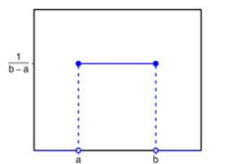
Figure 6-1
We may want to model the time it takes customer service to complete a call with the exponential distribution. See Figure 6-2.
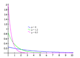
Figure 6-2
We may have standardized test scores that follow a bell-shaped curve like the Gaussian (Normal) Distribution. See Figure 6-3.

Figure 6-3

Figure 6-4
We may want to model the average time it takes for a component to be manufactured and use the bell-shaped Student t-distribution. See Figure 6-4.
This is just an introductory course so we are only going to cover a few distributions. If you want to explore more distributions, check out the chart by Larry Leemis at: http://www.math.wm.edu/~leemis/chart/UDR/UDR.html.
The probability of an interval between two X values is equal to the area under the density curve between those two \(X\) values. For a discrete random variable, we can assign probabilities to each outcome. We cannot do this for a continuous random variable. The probability for a single \(X\) value for a continuous random variable is 0. Thus “” are equivalent to “≤” and “≥.” In other words,
\[P(a ≤ X ≤ b) = P(a < X < b) = P(a ≤ X < b) = P(a < X ≤ b) \nonumber\]
since there is no area of a line.
We now will look at some specific models that have been found useful in practice. Consider an experiment that consists of observing events in a certain time frame, such as buses arriving at a bus stop or telephone calls coming into a switchboard during a specified period. It may then be of interest to place a probability distribution on the actual time of occurrence. In this section, we will tell you which distribution to use in the question.
6.02: Uniform Distribution
# Train arrival ~ Uniform(0, 15) minutes punif(10, 0, 15, lower.tail = FALSE) # P(X > 10) -> 0.3333 punif(8, 0, 15) - punif(2, 0, 15) # P(2 <= X <= 8) -> 0.4
The continuous uniform distribution models the probability that is the same on an interval from a to b. We use the following probability density function (PDF) to graph a straight line.
f(x)= \(\begin{cases}\frac{1}{b-a}, & \text { for } a \leq x \leq b \\ 0, & \text { elsewhere }\end{cases}\)
The probability is found by taking the area between two points within the rectangle formed from the x-axis, between the endpoints a and b, the length, and f(x) = 1/(b-a), the height. When working with continuous distributions it is helpful to draw a picture of the distribution, then shade in the area of the probability that you are trying to find. See Figure 6-5.

Figure 6-5
If a continuous random variable X has a uniform distribution with starting point a and ending point b then the distribution is denoted as X~U(a,b).
Area of a Rectangle = length*height
To find the probability (area) under the uniform distribution, use the following formulas.
- \(\mathrm{P}(X \geq x)=\mathrm{P}(X>x)=\left(\frac{1}{b-a}\right) \cdot(b-x)\)
- \(\mathrm{P}(X \leq x)=\mathrm{P}(X<x)=\left(\frac{1}{b-a}\right) \cdot(x-a)\)
- \(\mathrm{P}\left(x_{1} \leq X \leq x_{2}\right)=\mathrm{P}\left(x_{1}<X<x_{2}\right)=\left(\frac{1}{b-a}\right) \cdot\left(x_{2}-x_{1}\right)\)
The arrival time between trains at a train stop is uniformly distributed between 0 and 15 minutes. A student does not check the schedule and has arrived at the train stop.
- Compute the probability they wait more than 10 minutes.
- Compute the probability of waiting between 2 and 8 minutes.
Solution
a) First plug in the endpoints a = 0 and b = 15 into the PDF to get the height of the rectangle. The height is f(x)= \(\frac{1}{15-0}=\frac{1}{15}\). Draw and label the distribution with the a, b and the height as in Figure 6- 6. The probability is the area of the shaded rectangle P(X > 10). Draw a vertical line at x = 10. We want x values that are greater than 10, so shade the area to the right of 10, stopping at b = 15. To find the area of the shaded rectangle in Figure 6-6, we can take the length times the height. The length would be b – a = 15 – 10 = 5 and the height is f(x) = 1/15.

Figure 6-6
The area of the shaded rectangle is 5 (\(\frac{1}{15}\)) = \(\frac{1}{3}\) = 0.3333 or P(X > 10) = 0.3333, which is the probability of waiting more than 10 minutes. Note that this would be the same if we asked P(X ≥ 10) = 0.3333 since there is no area at the line X = 10.
b) The area will be length times height. Draw the picture and shade the rectangle between 2 and 8, see Figure 6-7. The length is b – a = 8 – 2 = 6 and the height is still f(x) = 1/15. P(2 ≤ X ≤ 8) = 6(\(\frac{1}{15}\)) = 0.4

Figure 6-7
6.03: Exponential Distribution
# Help time ~ Exponential, mean = 45 s (rate = 1/mean) pexp(120, rate = 1/45) # P(X < 120 s) -> 0.9305
An exponential distribution models a continuous random variable over time, area or space where the rate of occurrences decreases as X gets larger.
The probability density function (PDF) for an exponential curve is
\[f(x)= \{\begin{array}{l}\lambda e^{-x \lambda}, \text {for } x \geq 0 \\ 0, \text{elsewhere}\end{array}.\]
The value lambda λ is the fixed rate of occurrence and is equal to one divided by the mean, \(\frac{1}{\mu}\).
If the mean is given in the problem then you write the PDF as f(x)= \(\frac{1}{\mu} e^{\left(-\frac{x}{\mu}\right)}\), where e is a mathematical constant approximately equal to 2.71828, x ≥ 0 and x is the value you are trying to find the probability for, μ is the mean number of a successes over an interval of time, space, volume, etc. The distribution is denoted as X~Exp(λ).
Figure 6-8 gives example graphs for a mean of 5, 10 and 20. Note the curve hits the y-axis at 1/μ and keeps going forever to the right with an asymptote at y = 0.

Figure 6-8
You would need integral calculus skills to find the area under this curve. To get around having the calculus requirement, we have three scenarios that we can use to find probability for an exponential distribution where we will not have to use the PDF.
To find the probability (area) under the exponential curve, use the following formulas.
- \(\mathrm{P}(X \geq x)=\mathrm{P}(X>x)=\mathrm{e}^{-x / \mu}\)
- \(\mathrm{P}(X \leq x)=\mathrm{P}(X<x)=1-\mathrm{e}^{-x / \mu}\)
- \(\mathrm{P}\left(x_{1} \leq X \leq x_{2}\right)=\mathrm{P}\left(x_{1}<X<x_{2}\right)=e^{\left(-x_{1} / \mu\right)}-e^{\left(-x_{2} / \mu\right)}\)
The time it takes to help a customer at the customer service desk is exponentially distributed with an average help time of 45 seconds. Find the probability that a customer waits less than two minutes.
Solution
We need to have the same units as the mean in the question so instead of finding P(X < 2 minutes) we will use P(X < 120 seconds). Also note that < and ≤ find the same probabilities so use the equation \(\mathrm{P}(X
\[\mathrm{P}(X<120)=1-\mathrm{e}^{-120 / 45}=0.9305. \nonumber\]
In Excel use =EXPON.DIST(x,λ,TRUE) =EXPON.DIST(120,1/45,TRUE) = 0.9305.

Figure 6-9
Alternatively, as shown in Figure 6-9, the following website will calculate the exponential probability: https://homepage.divms.uiowa.edu/~mbognar/applets/exp.html.
6.04: Normal Distribution
Empirical Rule
Before looking at the process for finding the probabilities under a normal curve, recall the Empirical Rule that gives approximate values for areas under a bell-shaped distribution. The Empirical Rule, shown in Figure 6-10, is just an approximation for probability under any bell-shaped distribution and will only be used in this section to give you an idea of the size of the probability for different shaded areas. A more precise method for finding probabilities will be demonstrated using technology. Please do not use the empirical rule in the homework questions except for rough estimates.
The Empirical Rule (or 68-95-99.7 Rule)
In a bell-shaped distribution with mean μ and standard deviation σ,
- Approximately 68% of the observations fall within one standard deviation (σ) of the mean μ.
- Approximately 95% of the observations fall within two standard deviations (2σ) of the mean μ.
- Approximately 99.7% of the observations fall within three standard deviations (3σ) of the mean μ.

Gauss

Figure 6-10
For now, we will be working with the most common bell-shaped probability distribution known as the normal distribution, also called the Gaussian distribution, named after the German mathematician Johann Carl Friedrich Gauss. See Figure 6-11.

Figure 6-11
A normal distribution is a special type of distribution for a continuous random variable. Normal distributions are important in statistics because many situations in the real world have normal distributions.
Properties of the normal density curve:
- Symmetric bell-shaped.
- Unimodal (one mode).
- Centered at the mean μ= median = mode.
- The total area under the curve is equal to 1 or 100%.
- The spread of a normal distribution is determined by the standard deviation σ. The larger σ is, the more spread out the normal curve is from the mean.
- Follows the Empirical Rule.
If a continuous random variable X has a Normal distribution with mean μ and standard deviation σ then the distribution is denoted as X~N(μ, σ). Any x values from a Normal distribution can be transformed or standardized into a standard Normal distribution by taking the z-score of x.
The formula for the normal probability density function is: \(f(x)=\frac{1}{\sigma \sqrt{2 \pi}} e^{\left(-\frac{1}{2}\left(\frac{x-\mu}{\sigma}\right)^{2}\right)}\). We will not be using this formula.
The probability is found by using integral calculus to find the area under the PDF curve. Prior to the handheld calculators and personal computers, there were probability tables made to look up these areas. This text does not use probability tables and will instead rely on technology to compute the area under the curve.
Every time the mean or standard deviation changes the shape of the normal distribution changes. The center of the normal curve will be the mean and the spread of the normal curve gets wider as the standard deviation gets larger.
Figure 6-12 compares two normal distributions N(0, 1) in green on the left and N(7, 6) in blue on the right.

Figure 6-12
“‘So, what's odd about it?’
‘Nothing, it's Perfectly Normal.’”
(Adams, 2002)
6.4.1 Standard Normal Distribution
pnorm(1.39) # P(Z < 1.39) -> 0.9177 pnorm(1.68) - pnorm(-1.37) # P(-1.37 < Z < 1.68) -> 0.8682 pnorm(2) - pnorm(-2) # P(-2 < Z < 2) -> 0.9545 pnorm(1, lower.tail = FALSE) # P(Z > 1) -> 0.1587
Each link opens the Distributions panel pre-loaded on the standard normal — change the bound(s) to get the right tail P(Z>1) = 0.1587 too.
Opens XYZ Crunch with the values pre-loaded — change them and the result updates live.
A normal distribution with mean μ = 0 and standard deviation σ = 1 is called the standard normal distribution.
The letter Z is used exclusively to denote a variable that has a standard normal distribution and is written Z ~ N(0, 1). A particular value of Z is denoted z (lower-case) and is referred to as a z-score.
Recall that a z-score is the number of standard deviations x is from the mean. Anytime you are asked to find a probability of Z use the standard normal distribution.
Standardizing and z-scores:
A z-score is the number of standard deviations an observation x is above or below the mean μ. If the z-score is negative, x is below the mean. If the z-score is positive, x is above the mean.
If x is an observation from a distribution that has mean μ and standard deviation σ, the standardized value of x (or z-score) is \(\mathrm{z}=\frac{x-\mu}{\sigma}\).
To find the area under the probability density curve involves calculus so we will need to rely on technology to find the area.
Compute the area under the standard normal distribution to the left of z = 1.39.
Solution
First, draw a bell-shaped distribution with 0 in the middle as shown in Figure 6-13. Mark 1.39 on the number line and shade to the left of z = 1.39.

Figure 6-13
Note that the lower value of the shaded region is -∞, which the TI-84 does not have. Instead we use a really small number in scientific notation -1E99 or -1*1099 (make sure you use the negative sign (-) not the minus – sign.
The normalcdf on the calculator needs the lower and upper value of the shaded area followed by the mean and standard deviation. (The TI-89 uses -∞ for the lower boundary instead of -1E99.)
TI-84: Press [2nd] [DISTR] menu, select the normalcdf. Then type in the lower value, upper value, mean = 0, standard deviation = 1 to get normalcdf(-1E99,1.39,0,1) = 0.9177, which is your answer. The area under the curve is equivalent to the probability of getting a z-score less than 1.39, or P(Z < 1.39) = 0.9177.

TI-89: Go to the [Apps] Stat/List Editor, then select F5 [DISTR]. This will get you a menu of probability distributions. Arrow down to Normal Cdf and press [ENTER]. Enter the values for the lower z value (z1), upper z value (z2), μ = 0, and σ = 1 into each cell. Press [ENTER]. This is the cumulative distribution function and will return P(z1 < Z < z2). For a left-tail area use a lower bound of negative infinity (-∞), and for a right-tail area use an upper bound infinity (∞).

Excel: For Excel the program will only find the area to the left of a point. Therefore, if we want to find the area to the right of a point or between two points there will be one extra step. Use the formula =NORM.S.DIST(1.39,TRUE).
Compute the probability of getting a z-score between –1.37 and 1.68.
Solution
P(-1.37 ≤ Z ≤ 1.68) is the same as finding the area under the curve between –1.37 and 1.68. First, draw a bell-shaped distribution and identify the two points on the number line. Shade the area between the two points as shown in Figure 6-14.

Figure 6-14
TI Calculator: P(-1.37 ≤ Z ≤ 1.68) = normalcdf(-1.37,1.68,0,1) = 0.8682.
Excel: P(-1.37 ≤ Z ≤ 1.68) =NORM.S.DIST(1.68,TRUE)-NORM.S.DIST(-1.37,TRUE) = 0.8682.
Using Excel or TI-Calculator to Find Standard Normal Distribution
As you read through a problem look for some of the following key phrases in Figure 6-15. Once you find the phrase then match up to what sign you would use and then use the table to walk you through using Excel or the calculator. Note that we could also use the NORM.DIST function with µ = 0 and σ = 1.

Figure 6-15
Compute the area under the standard normal distribution that is 2 standard deviations from the mean.
Solution
A rough estimate using the Empirical Rule would be 0.95, however since this is not just any bell-shaped distribution, we will find the P(-2 ≤ Z ≤ 2). Draw and shade the curve as in Figure 6-16.
TI Calculator: P(-2 ≤ Z ≤ 2) = normalcdf(-2,2,0,1) = 0.9545.
Excel: P(-2 ≤ Z ≤ 2) =NORM.S.DIST(2,TRUE) -NORM.S.DIST(-2,TRUE) = 0.9545.

Figure 6-16
Compute the area to the right of z = 1.
Solution
Draw and shade the curve to find P(Z > 1). See Figure 6-17.
TI Calculator: P(Z > 1) = normalcdf(1,1E99,0,1) = 0.1587.
Excel: P(Z > 1) = 1-NORM.S.DIST(1,TRUE) = 0.1587.

Figure 6-17
6.4.2 Applications of the Normal Distribution
# 15-yr-old boys' heights ~ N(mean = 67, sd = 2.5) pnorm(69.5, 67, 2.5, lower.tail = FALSE) # P(X >= 69.5) -> 0.1587 # 2009 SAT math ~ N(501, 116) pnorm(600, 501, 116) - pnorm(400, 501, 116) # P(400 <= X <= 600) -> 0.6113
Pre-loaded on the raw mean and sd — no z-conversion, and the panel opens with the area already computed.
Opens XYZ Crunch with the values pre-loaded — change them and the result updates live.
Many variables are nearly normal, but none are exactly normal. Thus, the normal distribution, while not perfect for any single problem, is very useful for a variety of problems. Variables such as SAT scores and heights of United States adults closely follow the normal distribution. Note that the Excel function NORM.S.DIST is for a standard normal when µ = 0 and σ = 1
Using Excel or TI-Calculator to Find Normal Distribution Probabilities

Figure 6-18
TI-84: Press [2nd] [DISTR]. This will show a menu of probability distributions. Arrow down to 2:normalcdf( and press [ENTER]. This puts normalcdf( on the home screen. Enter the values for the lower x value (x1), upper x value (x2), μ, and σ with a comma between each. Press [ENTER]. This is the cumulative distribution function and will return P(x1 < X < x2). For example, to find P(80 < X < 110) when the mean is 100 and the standard deviation is 20, you should have normalcdf(80,110,100,20). If you leave out the μ and σ, then the default is the standard normal distribution. For a left-tail area use a lower bound of –1E99 (negative infinity), (press [2nd] [EE] to get E) and for a right-tail area use an upper bound of 1E99 (infinity). For example, to find P(Z < -1.37) you should have normalcdf(-1E99,-1.37).
TI-89: Go to the [Apps] Stat/List Editor, select F5 [DISTR]. This will show a menu of probability distributions. Arrow down to Normal Cdf and press [ENTER]. Enter the values for the lower x value (x1), upper x value (x2), μ, and σ into each cell. Press [ENTER]. This is the cumulative distribution function and will return P(x1 < X < x2). For example, to find P(80 < X < 110) when the mean is 100 and the standard deviation is 20, you should have in the following order 80, 110, 100, 20. If you have a z-score, use μ = 0 and σ = 1, then you will get a standard normal distribution. For a left-tail area use a lower bound of negative infinity (-∞), and for a right-tail area use an upper bound infinity (∞).
“The Hitchhiker's Guide to the Galaxy offers this definition of the word "Infinite." Infinite: Bigger than the biggest thing ever and then some. Much bigger than that in fact, really amazingly immense, a totally stunning size, "wow, that's big," time. Infinity is just so big that by comparison, bigness itself looks really titchy. Gigantic multiplied by colossal multiplied by staggeringly huge is the sort of concept we're trying to get across here.”
(Adams, 2002)
Let X be the height of 15-year old boys in the United States. Studies show that the heights of 15-year old boys in the United States are normally distributed with average height 67 inches and a standard deviation of 2.5 inches. Compute the probability of randomly selecting one 15-year old boy who is 69.5 inches or taller.
Solution
Find P(X ≥ 69.5) where X ~ N(67, 2.5). Draw the curve and label the mean, then shade the area to the right of 69.5.

Figure 6-19
First, standardize the value of x = 69.5 using the z-score formula \(z=\frac{x-\mu}{\sigma}\), where μ = 67 and σ = 2.5. The standardized value of x = 69.5 is \(z=\frac{69.5-67}{2.5}\) = 1.
Now using the standard normal distribution and shading the area to the right of z = 1 gives:
TI calculator: P(Z ≥ 1) = normalcdf(1,1E99,0,1) = 0.158655.
Excel: P(Z ≥ 1) = 1-NORM.S.DIST(1,TRUE) = 0.158655.

Figure 6-20
We could also use the Empirical rule to approximate P(X ≥ 69.5) because this is the same as being more than one standard deviation above the mean. Do you see why this makes sense?
If we were to add a standard deviation to 67 we would get 69.5. Thus P(X ≥ 69.5) \(\approx\) 0.16, which is close to our 15.87% using the standard normal distribution. The Empirical rule only gives an approximate value though.
The process of standardizing the X value was started so that we could use the standard normal distribution table to look up probabilities instead of using caclulus. With technology, you no longer have to standardize first, we can just find P(X ≥ 69.5).
TI calculator: P(X ≥ 69.5) = normalcdf(69.5, 1E99,67,2.5) \(\approx\) 0.158655 (The TI-89 use ∞ for the upper boundary instead of 1E99).
Excel: P(X ≥ 69.5) =1 – NORM.DIST(69.5,67,2.5,TRUE) = 0.158655.
Note that in Excel you can do this in two cells. First find the area to the left of 69.5 by using =NORM.DIST(69.5,67,2.5,TRUE) and the value 0.8413 is returned. In a new cell then subtract this value from 1 to get the answer 0.1587.

In 2009, the average SAT mathematics score was 501, with a standard deviation of 116. If we randomly selected a student from that year who took the SAT, what is the probability of getting a SAT mathematics score between 400 and 600?
Solution
Find P(400 ≤ X ≤ 600) using the TI calculator normalcdf(400,600,501,116) = 0.6113, which is also close to our results above. In Excel we can use the following formula =NORM.DIST(600,501,116,TRUE)- NORM.DIST(400,501,116,TRUE). Note that the right-hand endpoint goes in first. If you put the 400 in first you would get a negative answer, and probabilities are never negative. You can also do each piece separately in two cells, then in a third cell subtract the smaller area from the larger area.
A nice feature of this section is that the problems will say that the distribution is normally distributed, unlike the discrete distributions where you have to look for certain characteristics. However, when handling real data, you may have to know how to detect whether the data is normally distributed. One way to see if your variable is approximately normally distributed is by looking at a histogram, or we can use a normal probability plot.
6.4.3 Normal Probability Plot
# Points near the line => approximately normal set.seed(2) x <- rnorm(50, 67, 2.5) qqnorm(x); qqline(x)
A normal quantile plot, also called a normal probability plot, is a graph that is useful in assessing normality. A normal quantile plot plots the variable x against each of the x values corresponding z-score. It is not practical to make a normal quantile plot by hand.
Interpreting a normal quantile plot to see if a distribution is approximately normally distributed.
- All of the points should lie roughly on a straight line y = x.
- There should be no S pattern present.
- Outliers appear as points that are far away from the overall pattern of the plot.
Here are two examples of histograms with their corresponding quantile plots. Note that as the distribution becomes closer to a normal distribution the dots on the quantile plot will be in a straighter line. Figures 6-21 is the histogram and figure 6-22 is the corresponding normal probability plot. Note the histogram is skewed to the left and dots do not line up on the y = x line. Figures 6-23 and Figure 6-24 represent a sample that is approximately normally distributed. Note that the dots still do not line up perfectly on the line y = x, but they are close to the line.

Figure 6-21

Figure 6-22

Figure 6-23

Figure 6-24
6.4.4 Finding Percentiles for a Normal Distribution
qnorm(0.25) # 25th-pct z-score -> -0.6745 qnorm(0.90, 501, 116) # SAT top 10% cutoff -> 649.66 qnorm(c(0.01, 0.99), 246300, 15000) # middle 98% of home prices
Opens the inverse-normal mode pre-loaded; press Calculate for the score, then enter areas 0.01 / 0.99 on Normal(246300, 15000) for the middle-98% price bounds.
Opens XYZ Crunch with the values pre-loaded — change them and the result updates live.
Sometimes you will be given an area or probability and have to find the associated random variable x or z-score. For example, the probability below a point on the normal distribution is a percentile. If we find that the P(Z < 1.645) =NORM.S.DIST(1.645,TRUE) = 0.950015, that tells us that about 95% of z-scores are below 1.645. In other words, the z-score of 1.645 is the 95th percentile.
We can use technology to find z-score given a percentile. Most technology has built in commands that will find the probability below a point. If you want to find the area above a point, or between two points, then find the area below a point by using the complement rule and keep in mind that the total area under the curve is 1 and the total area below the mean is 0.5.
If x is an observation from a distribution that has mean μ and standard deviation σ, the standardized value of x (or zscore) is \(z=\frac{x-\mu}{\sigma}\).
If you have a z-score and want to convert back to x, you can do so by solving the above equation for x, which yields x = zσ + μ.
TI-84: Press [2nd] [DISTR]. This will get you a menu of probability distributions. Press 3 or arrow down to 3:invNorm( and press [ENTER]. This puts invNorm( on the home screen. Enter the area to the left of the x value, μ, and σ with a comma between each. Press [ENTER]. This will return the percentile for the x value. For example, to find the 95th percentile when the mean is 100 and the standard deviation is 20, you should have invNorm(0.95,100,20). If you leave out the μ and σ, then the default is the z-score for the standard normal distribution
TI-89: Go to the [Apps] Stat/List Editor, then select F5 [DISTR]. This will get you a menu of probability distributions. Arrow down to Inverse Normal and press [ENTER]. Enter the area to the left of the x value, μ, and σ into each cell. Press [ENTER]. This will return the percentile for the x value. For example, to find the 95th percentile when the mean is 100 and the standard deviation is 20, you should enter 0.95, 100, 20.

If you use μ = 0 and σ = 1, then the default is the z-score for the standard normal distribution.
Compute the z-score that corresponds to the 25th percentile.
Solution
First, draw the standard normal curve with zero in the middle as in Figure 6-25. The 25th percentile would have to be below the mean since the mean = median = 50th percentile for a bell-shaped distribution.

Figure 6-25

It is okay if you do not have this drawing to scale, but drawing a picture similar to Figure 6-25 will give you a good idea if your answer is correct. For instance, by just looking at this graph we can see that the answer for the z-score will need to be a negative number.
TI Calculator: z = invNorm(0.25,0,1) = -0.6745.
Excel: z = NORM.S.INV(0.25) = -0.6745.
The z = -0.6745 represents the 25th percentile.
Compute the z-score that corresponds to the area of 0.4066 between zero and z shown in Figure 6-26.
Solution
First notice that this picture does not quite match the calculator or Excel, which will only find for a left-tail area. The value of zero is the median on a standard normal distribution, so 50% of the area lies to the left of z = 0. This means that the total area to the left of the unknown z-score would be 0.5 + 0.4066 = 0.9066.

Figure 6-26
TI Calculator: z = invNorm(0.9066) = 1.32.
Excel: z = NORM.S.INV(0.9066) = 1.32.
Using Excel or TI-Calculator for the Percentile of a Normal Distribution
Note that the NORM.S.INV function is for a standard normal when µ = 0 and σ = 1.

Figure 6-27
In 2009, the average SAT mathematics score was 501, with a standard deviation of 116. Find the SAT score that is for the top 10% of students taking the exam that year.
Solution
Draw the distribution curve and shade the top 10% as shown in Figure 6- 28. The area below the unknown x value in Figure 6-28 is 1 – 0.10 = 0.90.

Figure 6-28
TI Calculator: invNorm(0.9,501,116) = 649.66.
Excel: =NORM.INV(0.9,501,116) = 649.66.
A student that scored above 649.66 would be in the top 10%, also known as the 90th percentile.
We could have also found the z-score that corresponds to the top 10%. Then use the z-score formula to find the xvalue. Using Excel =NORM.S.INV(0.9) = 1.2816. Then use the formula x = zσ + μ = 1.2816 ∙ 116 + 501 = 649.67. This is using a rounded z-score so the answer is slightly off, but close.
Note: It is common practice to round z-scores to two decimal places. This is left over from using probability tables that only went out to two decimal places. If you use a rounded z-score in other calculations then keep in mind that you will get a larger rounding error.
If the average price of a new one family home is $246,300 with a standard deviation of $15,000, find the minimum and maximum prices of the houses that a contractor will build to satisfy the middle 98% of the market. Assume that the variable is normally distributed.
Solution
First, draw the curve and shade the middle area of 0.98, see Figure 6-29. We need to get the area to the left of the x1 value. Take the complement 1 – 0.98 = 0.02, then split this area between both tails.
The lower tail area for x1 would have 0.02/2 = 0.01. The upper value of x2 will have a left tail area of 0.99.

Figure 6-29
On the calculator use, invNorm(0.01,246300,15000) and you get a minimum price of $211404.78 and use invNorm(0.99,246300,15000) and you get a maximum price of $281195.22.
In Excel you would have to do this in two separate cells =NORM.INV(0.01,246300,15000) = $211,404.78 and =NORM.INV(0.99,246300,15000) = $281,195.22.
6.05: The Central Limit Theorem
mu <- 57337; sigma <- 7500 pnorm(55000, mu, sigma) # one teacher -> 0.3777 pnorm(55000, mu, sigma/sqrt(10)) # mean of n=10 -> 0.1622 pnorm(55000, mu, sigma/sqrt(100)) # mean of n=100 -> 0.00092
# Simulate the sampling distribution of x-bar: N(67, 2.5), n = 16 set.seed(1) xbar <- replicate(10000, mean(rnorm(16, 67, 2.5))) c(mean = mean(xbar), sd = sd(xbar)) # ~67 and ~0.625 hist(xbar, main = "Sampling distribution of x-bar (n = 16)")
Pre-loaded with one teacher (sd 7500): P(X<55000) = 0.3777. Re-enter the sd as 7500/√10 = 2371.71, then 7500/√100 = 750, and watch P fall to 0.1622 → 0.00092.
Opens XYZ Crunch with the values pre-loaded — change them and the result updates live.
The sample mean, denoted \(\overline{ x }\), is the average of a sample of a variable X. The sample mean is an estimate of the population mean µ. Every sample has a sample mean and these sample means differ (depending on the sample). Thus, before a sample is selected \(\overline{ x }\) is a variable, in fact, if the sample is a random sample then \(\overline{ x }\) is a random variable. For this reason, we can think of the “distribution of \(\overline{ x }\),” called the “Sampling Distribution of \(\overline{ x }\),” as the theoretical histogram constructed from the sample averages of all possible samples of size n.Definition: Word
Mean and Standard Deviation of a Sample Mean
Let \(\overline{ x }\) be the mean of a random sample of size n from a population having mean μ and standard deviation σ, then
The mean of the sample means = \(\mu_{\bar{x}}\) = µ.
The standard deviation (standard error) of the sample means = \(\sigma_{\bar{x}}=\frac{\sigma}{\sqrt{n}}\).
This says that the mean of the sample means is the same as the population mean. The standard deviation of the sample means is the population standard deviation divided by the square root of the sample size. This is called the sampling distribution of the mean.
Let X be the height of men in the United States. Studies show that the heights of 15-year old boys in the United States are normally distributed with average height 67 inches and a standard deviation of 2.5 inches. A random experiment consists of choosing 16 15-year old boys at random. Compute the mean and standard deviation of \(\overline{ x }\), that is, the mean and standard deviation for the average height of a random sample of 16 boys.
Solution
The mean of the sample means is the same as the population mean \(\mu_{\bar{x}}\) = 67.
The standard deviation in the sample means is the population standard deviation divided by the square root of the sample size, \(\sigma_{\bar{x}}=\frac{\sigma}{\sqrt{n}}=\frac{2.5}{\sqrt{16}}=0.625\).
Notice that the mean of a sample means is always the same as the mean of the population, but the standard deviation is smaller. See Figure 6-30.
Sampling Distribution of a Sample Mean
If a population is normally distributed N(µ, σ), then the sample mean \(\overline{ x }\) of n independent observations is normally distributed as \(N\left(\mu, \frac{\sigma}{\sqrt{n}}\right)\) /
Figure 6-31 shows three population distributions and the corresponding sampling distributions for sample sizes of 2, 5, 12 and 30. Notice as the sample size gets larger, the sampling distribution gets closer to the dashed red line of the normal distribution. Video explanation of this process: https://youtu.be/lsCc_pS3O28.

Retrieved from OpenIntroStatistics.
Figure 6-31
The Central Limit Theorem establishes that in some situations the distribution of the sample statistic will take on a normal distribution, even when the population is not normally distributed. This allows us to use the normal distribution to make inferences from samples to populations.
The Central Limit Theorem guarantees that the distribution of the sample mean will be normally distributed when the sample size is large (usually 30 or higher) no matter what shape the population distribution is.
Finding Probabilities Using the Central Limit Theorem (CLT)
If we are finding the probability of a sample mean and have a sample size of 30 or more, or the population was normally distributed, then we can use the normal distribution to find the probability that the sample mean is below, above or between two values using the CLT.
Watch this video on using this applet for the Central Limit Theorem, and then take some time to play with the applet to get a sense of the difference between the distribution of the population, the distribution of a sample and the sampling distribution.
Watch the video on how to use the applet: https://youtu.be/aIPvgiXyBMI.
Try the applet on your own. Applet: http://onlinestatbook.com/stat_sim/sampling_dist/index.html.
The population of midterm scores for all students taking a PSU Business Statistics course has a known standard deviation of 5.27. The mean of the population is 18.07 and the median of the population is 19. A sample of 25 was taken and the sample mean was 18.07 and we want to know what the sampling distribution for the mean looks like. Figure 6-32 shows 3 graphs using the Sampling Distribution Applet.
a) What is the mean and standard deviation of the sampling distribution? b) Would you expect midterm exam scores to be skewed or bell-shaped? c) Which of these graphs in Figure 6-32 correspond to the distribution of the population, distribution of a single sample and the sampling distribution of the mean? d) Compute the probability that for next term’s class they have a sample mean of more than 20. a) By the Central Limit Theorem (CLT) the mean of the sampling distribution \(\mu_{\bar{x}}\) equals the mean of the population which was given as µ=18.07. The standard deviation of the sampling distribution by the CLT would be the population standard deviation divided by the square root of the sample size \(\sigma_{\bar{x}}=\frac{\sigma}{\sqrt{n}}=\frac{5.27}{\sqrt{25}}=1.054\) b) The population mean = 18.07 is smaller than the median = 19 therefore the distribution is negatively skewed, the mean is pulled in the direction of the outliers. c) Using the Sampling Distribution Applet and the CLT, the sampling distribution will be bell-shaped therefore, graph 3 has to be the sampling distribution. Graphs 1 & 2 in Figure 6-32 are both negatively skewed. A single sample of 25 should look similar to the entire population, but we would expect only 25 items and not every score possible would be received from the 25 students. Graph 1 in Figure 6-32 fits this description and therefore the graph of the distribution of a single sample (which is not the same thing as the sampling distribution) is graph 1. This leaves graph 2 as the distribution of the population. Figure 6-33 is a picture of the applet modeling the exam scores. Note the top picture is the population distribution, the second graph is simulating a single sample drawn and the bottom picture is a graph of all the sample means for each sample. This last graph is the sampling distribution of the means. d) The P(\(\bar{X}\) > 20) would be normally distributed with a mean \(\mu_{\bar{x}}\) = 18.07 with a standard deviation of \(\sigma_{\bar{x}}=\frac{\sigma}{\sqrt{n}}=\frac{5.27}{\sqrt{25}}=1.054\) Draw and shade the sampling distribution curve. This calculator can be used to draw and shade the sampling distribution: http://homepage.divms.uiowa.edu/~mbognar/applets/normal.html, filling in the mean μ, standard deviation \(\frac{\sigma}{\sqrt{n}}\) and x-value (in this case the sample mean) will find the probability. See Figure 6-34. TI Calculator: normalcdf(20,1E99,18.07,5.27/√25) = 0.0335. Excel: P(\(\bar{X}\) > 20) =1-NORM.DIST(20,18.07,5.27/SQRT(25),TRUE) = 0.0335.
Solution
Let X be the height of 15-year old boys in the United States. Studies show that the heights of 15-year old boys in the United States are normally distributed with average height of 67 inches and a standard deviation of 2.5 inches. A random experiment consists of randomly choosing sixteen 15-year old boys. Compute the probability that the mean height of those sampled is 69.5 inches or taller.
Solution
The sample mean \(\mu_{\bar{x}}\) is approximately \(N(67,0.625) . \mathrm{P}(\bar{X} \geq 69.5)=P\left(\frac{8-67}{0.625} \geq \frac{69.5-67}{0.625}\right)=\mathrm{P}(Z \geq 4) \approx 0.00003\), using the calculator, be careful with the scientific notation. This is a very small probability.

This should make sense because one would think that the likelihood of randomly selecting 16 boys that have an average height of 5’9.5” would be slim.
Figure 6-35 shows the density curves showing the shaded areas of P(X ≥ 69.5) and P(\(\mu_{\bar{x}}\) ≥ 69.5).
The sampling distribution has a much smaller spread (standard deviation) and hence less area to the right of 69.5.
In general, the Central Limit Theorem questions will use the same method as previous sections, however you will use a standard deviation of \(\frac{\sigma}{\sqrt{n}}\) and a z-score of \(z=\frac{\bar{x}-\mu}{\left(\frac{\sigma}{\sqrt{n}}\right)}\).
The average teacher’s salary in Connecticut (ranked first among states) is $57,337. Suppose that the distribution of salaries is normally distributed with a standard deviation of $7,500.
a) What is the probability that a randomly selected teacher makes less than $55,000 per year?
b) If we sample 10 teachers’ salaries, what is the probability that the sample mean is less than $55,000?
c) If we sample 100 teachers’ salaries, what is the probability that the sample mean is less than $55,000?
Solution
a) Find P(X < 55000), since we are only looking at one person use \(z=\frac{x-\mu}{\sigma}\). If we were asked to standardize the salary, \(z=\frac{55000-57337}{7500}=-0.3116\), however we can use technology and skip this step.
Use the normalcdf(-1E99,55000,57337,7500) (the TI-89 use -∞ for the lower boundary instead of -1E99) and you get the probability of 0.3777. The P(X < 55000) = P(Z < –0.3116) = 0.3777.
Note that we are not using the CLT since we are not finding the probability of an average for a group of people, just the probability for one person.

b) Find P(\(\mu_{\bar{x}}\) < 55000), but we are looking at the probability of a mean for 10 teachers, so use \(z=\frac{\bar{x}-\mu}{\left(\frac{\sigma}{\sqrt{n}}\right)}\). Standardize the salary, \(z=\frac{55000-57337}{\left(\frac{7500}{\sqrt{10}}\right)}=–0.9853657189\), use your calculator to get P(\(\mu_{\bar{x}}\) < 55000) = P(Z < –0.9853657189) = 0.1622.
You do not need the extra step of finding the z-score first. Instead you can use normalcdf(-1E99,55000,57337,7500/√10) = 0.1622.

c) Find P(\(\mu_{\bar{x}}\) < 55000), but we are looking at the probability of a mean for 100 teachers, so use \(z=\frac{\bar{x}-\mu}{\left(\frac{\sigma}{\sqrt{n}}\right)}\). Standardize the salary, \(z=\frac{55000-57337}{\left(\frac{7500}{\sqrt{100}}\right)}=–3.116\) use your calculator normalcdf(-1E99,55000,57337,7500/√100) to get P(\(\mu_{\bar{x}}\) < 55000) = P(Z < –3.116) = 0.0009167.

As the sample size increase, the probability of seeing a sample mean of less than $55,000 is getting smaller.
When you have a z-score that is less than –3 or greater than 3 we would call this a rare event or outlier. We will use this same process in inferential statistics in chapter 8.
6.06: Chapter 6 Exercises
1. The waiting time for a bus is uniformly distributed between 0 and 15 minutes. What is the probability that a person has to wait at most 8 minutes for a bus?
2. The distance a golf ball travels when hit by a driver club is uniformly distributed between 200 and 300 feet. What is the probability that the ball hit by a driver club with travel at least 280 feet?
3. The time it takes me to wash the dishes is uniformly distributed between 7 minutes and 16 minutes. What is the probability that washing dishes tonight will take me between 9 and 14 minutes?
4. Bus wait times are uniformly distributed between 5 minutes and 18 minutes. Compute the probability that a randomly selected bus wait time will be between 9 and 13 minutes.
5. The lengths of an instructor’s classes have a continuous uniform distribution between 60 and 90 minutes. If one such class is randomly selected, find the probability that the class length is less than 70.7 minutes.
6. The time it takes for students to finish an exam is uniformly distributed between 1 to 2 hours. What is the probability that a randomly selected students finishes their exam in at least 95 minutes?
7. Suppose the commuter trains of a public transit system have a waiting time during peak rush hour periods of fifteen minutes. Assume the waiting times are uniformly distributed. Find the probability of waiting between 7 and 8 minutes.
8. Suppose that elementary students' ages are uniformly distributed from 5 to 13 years old. Compute the probability that a randomly selected elementary student will be between ages 7.07 and 10.33 years old.
9. The amount of gasoline sold daily at a service station is uniformly distributed with a minimum of 2,000 gallons and a maximum of 5,000 gallons.
a) Compute the probability that the service station will sell at least 4,000 gallons?
b) Compute the probability that daily sales will fall between 2,500 and 3,000 gallons?
c) What is the probability that the station will sell exactly 2,500 gallons?
10. The sojourn time (waiting time plus service time) for customers waiting at a movie theater box office is exponentially distributed with a mean of 4 minutes. Find the following.
a) The probability that the sojourn time will be more than 5 minutes.
b) The probability that the sojourn time will be less than 5 minutes.
c) The probability that the sojourn time will be at most 5 minutes.
11. Suppose that the distance, in miles, that people are willing to commute to work is exponentially distributed with mean 24 miles. What is the probability that people are willing to commute at most 12 miles to work?
12. On average, a pair of running shoes lasts 13 months if used every day. The length of time running shoes last is exponentially distributed. What is the probability that a pair of running shoes last less than 6 months if used every day?
13. The lifetime of a light emitting diode (LED) lightbulb is exponentially distributed with an average lifetime of 5,000 hours. Find the following.
a) The probability that the LED lightbulb will last more than 3,500 hours.
b) The probability that the LED lightbulb will last less than 4,000 hours.
c) The probability that the LED lightbulb will last between 3,500 and 4,500 hours.
14. The number of days ahead travelers purchase their airline tickets can be modeled by an exponential distribution with the average amount of time equal to 50 days.
a) Compute the probability that a traveler purchases a ticket no more than 85 days ahead of time.
b) Compute the probability that a traveler purchases a ticket more than 90 days ahead of time.
c) Compute the probability that a traveler purchases a ticket within 85 and 90 days ahead of the flight date.
15. The average time it takes a salesperson to finish a sale on the phone is 5 minutes and is exponentially distributed.
a) Compute the probability that less than 10 minutes pass before a sale is completed.
b) Compute the probability that more than 15 minutes pass before a sale is completed.
c) Compute the probability that between 10 and 15 minutes pass before a sale is completed.
16. A brand of battery is advertised to last 3 years. Assume the advertised claim is true and that the time the battery lasts is exponentially distributed. What is the probability that one of these batteries will last within 15 months of the advertised average?
17. For a standard normal distribution, find the following probabilities.
a) P(Z > -2.06)
b) P(-2.83 < Z < 0.21)
c) P(Z < 1.58) d) P(Z ≥ 1.69)
e) P(Z < -2.82)
f) P(Z > 2.14)
g) P(1.97 ≤ Z ≤ 2.93)
h) P(Z ≤ -0.51)
18. Compute the following probabilities where Z ~ N(0,1).
a) P(Z < 1.57)
b) P(Z > -1.24)
c) P(-1.96 ≤ Z ≤ 1.96)
d) P(Z ≤ 3)
e) P(1.31 < Z < 2.15)
f) P(Z ≥ 1.8)
19. Compute the following probabilities where Z ~ N(0,1).
a) P(Z ≤ -2.03)
b) P(Z > 1.58)
c) P(-1.645 ≤ Z ≤ 1.645)
d) P(Z < 2)
e) P(-2.38 < Z < -1.12)
f) P(Z ≥ -1.75)
20. Compute the area under the standard normal distribution to the left of z = -1.05.
21. Compute the area under the standard normal distribution to the left of z = -0.69.
22. Compute the area under the standard normal distribution to the right of z = 2.08.
23. Compute the area under the standard normal distribution to the right of z = 1.22.
24. Compute the area under the standard normal distribution between z = -0.29 and z = 0.14.
25. Compute the area under the standard normal distribution between z = -2.97 and z = -2.14.
26. Compute the area under the curve of the standard normal distribution that is within 1.328 standard deviations from either side of the mean.
27. Compute the area under the standard normal distribution to the left of z = 0.85.
28. Compute the z-score that has an area of 0.85 to the left of the z-score.
29. For the standard normal distribution, find the z-score that gives the 29th percentile.
30. For the standard normal distribution, find the z-score that gives the 75th percentile.
31. Compute the two z-scores that give the middle 99% of the standard normal distribution.
32. Compute the two z-scores that give the middle 95% of the standard normal distribution.
33. Find the IQR for the standard normal distribution.
34. The length of a human pregnancy is normally distributed with a mean of 272 days with a standard deviation of 9 days (Bhat & Kushtagi, 2006).
a) Compute the probability that a pregnancy lasts longer than 281 days.
b) Compute the probability that a pregnancy lasts less than 250 days.
c) How many days would a pregnancy last for the shortest 20%?
35. Arm span is the physical measurement of the length of an individual's arms from fingertip to fingertip. A man’s arm span is approximately normally distributed with mean of 70 inches with a standard deviation of 4.5 inches.
a) Compute the probability that a randomly selected man has an arm span below 65 inches.
b) Compute the probability that a randomly selected man has an arm span between 60 and 72 inches.
c) Compute the length in inches of the 99th percentile for a man’s arm span.
36. The size of fish is very important to commercial fishing. A study conducted in 2012 found the length of Atlantic cod caught in nets in Karlskrona to have a mean of 49.9 cm and a standard deviation of 3.74 cm (Ovegard, Berndt & Lunneryd, 2012). Assume the length of fish is normally distributed.
a) Compute the probability that a cod is longer than 55 cm.
b) What is the length in cm of the longest 15% of Atlantic cod in this area?
37. A dishwasher has a mean life of 12 years with an estimated standard deviation of 1.25 years ("Appliance life expectancy," 2013). Assume the life of a dishwasher is normally distributed.
a) Compute the probability that a dishwasher will last less than 10 years.
b) Compute the probability that a dishwasher will last between 8 and 10 years.
c) Compute the number of years that the bottom 25% of dishwashers would last.
38. The price of a computer is normally distributed with a mean of $1400 and a standard deviation of $60.
a) What is the probability that a buyer paid less than $1220?
b) What is the probability that a buyer paid between $1400 and $1580?
c) What is the probability that a buyer paid more than $1520?
d) What is the probability that a buyer paid between $1340 and $1460?
e) What is the probability that a buyer paid between $1400 and $1520?
f) What is the probability that a buyer paid between $1400 and $1460?
39. Heights of 10-year-old children, regardless of sex, closely follow a normal distribution with mean 55.7 inches and standard deviation 6.8 inches.
a) Compute the probability that a randomly chosen 10-year-old child is less than 50.4 inches.
b) Compute the probability that a randomly chosen 10-year-old child is more than 59.2 inches.
c) What proportion of 10-year-old children are between 50.4 and 61.5 inches tall?
d) Compute the 85th percentile for 10-year-old children.
40. The mean yearly rainfall in Sydney, Australia, is about 137 mm and the standard deviation is about 69 mm ("Annual maximums of," 2013). Assume rainfall is normally distributed. How many yearly mm of rainfall would there be in the top 25%?
41. The mean daily milk production of a herd of cows is assumed to be normally distributed with a mean of 33 liters, and standard deviation of 10.3 liters. Compute the probability that daily production is more than 40.9 liters?
42. The amount of time to complete a physical activity in a PE class is normally distributed with a mean of 33.2 seconds and a standard deviation of 5.8 seconds. Round answers to 4 decimal places.
a) What is the probability that a randomly chosen student completes the activity in less than 28.9 seconds?
b) What is the probability that a randomly chosen student completes the activity in more than 37.2 seconds?
c) What proportion of students take between 28.5 and 37.3 seconds to complete the activity? d) 70% of all students finish the activity in less than _____ seconds.
43. A study was conducted on students from a particular high school over the last 8 years. The following information was found regarding standardized tests used for college admittance. Scores on the SAT test are normally distributed with a mean of 1023 and a standard deviation of 204. Scores on the ACT test are normally distributed with a mean of 19.3 and a standard deviation of 5.2. It is assumed that the two tests measure the same aptitude, but use different scales.
a) Compute the SAT score that is the 50-percentile.
b) Compute the ACT score that is the 50-percentile.
c) If a student gets an SAT score of 1288, find their equivalent ACT score. Go out at least 5 decimal places between steps.
44. Delivery times for shipments from a central warehouse are exponentially distributed with a mean of 1.73 days (note that times are measured continuously, not just in number of days). The standard deviation of an exponential distribution is equal to the mean of 1.73 days. A random sample of 108 shipments are selected and their shipping times are observed. Use the Central Limit Theorem to find the probability that the mean shipping time for the 108 shipments is less than 1.53 days.
45. The MAX light rail in Portland, OR has a waiting time that is uniformly distributed with a mean waiting time of 5 minutes with a standard deviation of 2.9 minutes. A random sample of 40 wait times was selected. What is the probability the sample mean wait time is under 4 minutes?
46. The average credit card debt back in 2016 was $16,061 with a standard deviation of $4100. What is the probability that a sample of 35 people owe a mean of more than $18,000?
47. A certain brand of electric bulbs has an average life of 300 hours with a standard deviation of 45. A random sample of 100 bulbs is tested. What is the probability that the sample mean will be less than 295?
48. Assume that the birth weights of babies are normally distributed with a mean of 3363 grams and a standard deviation of 563 grams.
a) Compute the probability that a randomly selected baby weighs between 3200 grams and 3600 grams.
b) Compute the probability that the average weight of 30 randomly selected babies is between 3200 grams and 3600 grams.
c) Why did the probability increase?
49. If the Central Limit Theorem is applicable, this means that the sampling distribution of a __________ population can be treated as normal since the __________ is __________.
a) symmetrical; variance; large
b) positively skewed; sample size; small
c) negatively skewed; standard deviation; large
d) non-normal; mean; large
e) negatively skewed; sample size; large
50. Match the following 3 graphs with the distribution of the population, the distribution of the sample, and the sampling distribution.
a) Distribution of the Population
b) Distribution of the Sample
c) Sampling Distribution
i. 
ii. 
iii. 
51. Match the following 3 graphs with the distribution of the population, the distribution of the sample, and the sampling distribution.
a) Distribution of the Population
b) Distribution of the Sample
c) Sampling Distribution
i. 
ii. 
iii. 
52. Match the following 3 graphs with the distribution of the population, the distribution of the sample, and the sampling distribution.
a) Distribution of the Population
b) Distribution of the Sample
c) Sampling Distribution
i. 
ii. 
iii. 
6.07: Chapter 6 Formulas
|
Uniform Distribution \(f(x)=\frac{1}{b-a}, \text { for } a \leq x \leq b\)
|
Exponential Distribution \(f(x)=\frac{1}{\mu} e^{\left(-\frac{x}{\mu}\right)}, \text { for } x \geq 0\)
|
|
Standard Normal Distribution \(\mu=0, \sigma=1\) |
Central Limit Theorem \(Z \text {-score: } z=\frac{\bar{x}-\mu}{\left(\frac{\sigma}{\sqrt{n}}\right)}\) |
| Normal Distribution Probabilities: |
P(X ≤ x) = P(X < x)
Excel: =NORM.DIST(x,µ,σ,true) TI-84: normalcdf(-1E99,x,µ,σ) |
|
P(X ≥ x) = P(X > x)
Excel: = 1–NORM.DIST(x,µ,σ,true) TI-84: normalcdf(x,1E99,µ,σ) |
P(x1 ≤ X ≤ x2) = P(x1 < X < x2) =
Excel: =NORM.DIST(x2,µ,σ,true)- NORM.DIST(x1,µ,σ,true) TI-84: normalcdf(x1,x2,µ,σ) |
| Percentiles for Normal Distribution: |
P(X ≤ x) = P(X < x)
Excel: =NORM.INV(area,µ,σ) TI-84: invNorm(area,µ,σ) |
|
P(X ≥ x) = P(X > x)
Excel: =NORM.INV(1–area,µ,σ) TI-84: invNorm(1–area,µ,σ) |
P(x1 ≤ X ≤ x2) = P(x1 < X < x2) =
Excel: x1 =NORM.INV((1–area)/2,µ,σ) x2 =NORM.INV(1–((1–area)/2),µ,σ) TI-84: x1 = invNorm((1–area)/2,µ,σ) x2 =invNorm(1–((1–area)/2),µ,σ) |
From Mostly Harmless Statistics by Rachel L. Webb, adapted from LibreTexts. Licensed CC BY-SA 4.0. XYZ Homework OER web edition, adapted with 7 verified corrections (see errata).


