
6.1 Introductions
A continuous random variable (usually denoted as X) is a variable that has an infinite number of random values in an interval of numbers. There are many different types of continuous distributions. To be a valid continuous distribution the total area under the curve has to be equal to one and the function’s y-values need to be positive.
For example, we may have a random variable that is uniformly distributed so we could use the Uniform distribution that looks like a rectangle. See Figure 6-1.
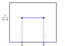
Figure 6-1
We may want to model the time it takes customer service to complete a call with the exponential distribution. See Figure 6-2.
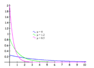
Figure 6-2
We may have standardized test scores that follow a bell-shaped curve like the Gaussian (Normal) Distribution. See Figure 6-3.
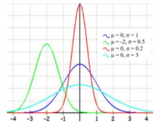
Figure 6-3
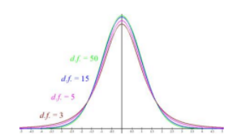
Figure 6-4
We may want to model the average time it takes for a component to be manufactured and use the bell-shaped Student t-distribution. See Figure 6-4.
This is just an introductory course so we are only going to cover a few distributions. If you want to explore more distributions, check out the chart by Larry Leemis at: http://www.math.wm.edu/~leemis/chart/UDR/UDR.html.
Very Important
The probability of an interval between two X values is equal to the area under the density curve between those two values. For a discrete random variable, we can assign probabilities to each outcome. We cannot do this for a continuous random variable. The probability for a single value for a continuous random variable is 0. Thus “” are equivalent to “≤” and “≥.” In other words,
since there is no area of a line.
We now will look at some specific models that have been found useful in practice. Consider an experiment that consists of observing events in a certain time frame, such as buses arriving at a bus stop or telephone calls coming into a switchboard during a specified period. It may then be of interest to place a probability distribution on the actual time of occurrence. In this section, we will tell you which distribution to use in the question.
Adapted from Mostly Harmless Statistics by Rachel Webb (Portland State University, https://mostlyharmlessstat.wixsite.com/webpage), © Rachel Webb, licensed under CC BY-SA 4.0. Changes were made. License: CC-BY-SA-4.0.