Mostly Harmless StatisticsXYZ Homework Edition

⇩ Download ▾

6.7 Chapter 6 Formulas

Uniform Distribution f(x)=1ba, for axbf(x)=\frac{1}{b-a}, \text { for } a \leq x \leq b P(Xx)=P(X>x)=(1ba)·(bx){P}(X \geq x)=\mathrm{P}(X>x)=\left(\frac{1}{b-a}\right) \cdot(b-x) P(Xx)=P(X<x)=(1ba)·(xa)\mathrm{P}(X \leq x)=\mathrm{P}(X<x)=\left(\frac{1}{b-a}\right) \cdot(x-a) P(x1Xx2)=P(x1<X<x2)=(1ba)·(x2x1){P}\left(x_{1} \leq X \leq x_{2}\right)=\mathrm{P}\left(x_{1}<X<x_{2}\right)=\left(\frac{1}{b-a}\right) \cdot\left(x_{2}-x_{1}\right) Exponential Distribution f(x)=1μe(xμ), for x0f(x)=\frac{1}{\mu} e^{\left(-\frac{x}{\mu}\right)}, \text { for } x \geq 0 P(Xx)=P(X>x)=ex/μ\mathrm{P}(X \geq x)=\mathrm{P}(X>x)=\mathrm{e}^{-x / \mu} P(Xx)=P(X<x)=1ex/μ\mathrm{P}(X \leq x)=\mathrm{P}(X<x)=1-\mathrm{e}^{-x / \mu} P(x1Xx2)=P(x1<X<x2)=e(x1μ)e(x2μ)\mathrm{P}\left(x_{1} \leq X \leq x_{2}\right)=\mathrm{P}\left(x_{1}<X<x_{2}\right)=e^{\left(-\frac{x_{1}}{\mu}\right)}-e^{\left(-\frac{x_{2}}{\mu}\right)}
Standard Normal Distribution μ=0,σ=1\mu=0, \sigma=1
z-score: z=xμσz \text {-score: } z=\frac{x-\mu}{\sigma}
x=zσ+μx=z \sigma+\mu
Central Limit Theorem Z-score: z=x¯μ(σn)Z \text {-score: } z=\frac{\bar{x}-\mu}{\left(\frac{\sigma}{\sqrt{n}}\right)}
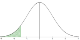
Normal Distribution Probabilities: P(X ≤ x) = P(X < x) Bell curve with the left-tail area below a value left of the mean shaded green, illustrating the left-tail probability P(X <= x). Excel: =NORM.DIST(x,µ,σ,true) TI-84: normalcdf(-1E99,x,µ,σ)
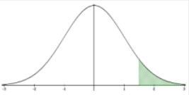
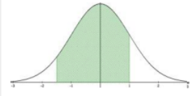
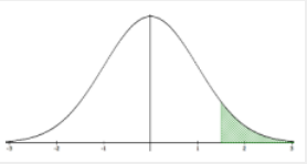
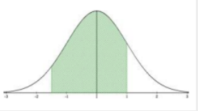
P(X ≥ x) = P(X > x) Bell curve with the right-tail area above a value right of the mean shaded green, illustrating the right-tail probability P(X >= x). Excel: = 1–NORM.DIST(x,µ,σ,true) TI-84: normalcdf(x,1E99,µ,σ) P(x1 ≤ X ≤ x2) = P(x1 < X < x2) = Bell curve with the central area between two values on either side of the mean shaded green, illustrating the between probability P(x1 <= X <= x2). Excel: =NORM.DIST(x2,µ,σ,true)- NORM.DIST(x1,µ,σ,true) TI-84: normalcdf(x1,x2,µ,σ)
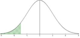
Percentiles for Normal Distribution: P(X ≤ x) = P(X < x) Bell curve with the left-tail area shaded green, illustrating the percentile case of finding the x-value with a given area to its left, P(X <= x). Excel: =NORM.INV(area,µ,σ) TI-84: invNorm(area,µ,σ)
P(X ≥ x) = P(X > x) Bell curve with the right-tail area shaded green, illustrating the percentile case of finding the x-value with a given area to its right, P(X >= x). Excel: =NORM.INV(1–area,µ,σ) TI-84: invNorm(1–area,µ,σ) P(x1 ≤ X ≤ x2) = P(x1 < X < x2) = Bell curve with the middle area between two values shaded green, illustrating finding the two x-values x1 and x2 that bound a given central area. Excel: x1 =NORM.INV((1–area)/2,µ,σ) x2 =NORM.INV(1–((1–area)/2),µ,σ) TI-84: x1 = invNorm((1–area)/2,µ,σ) x2 =invNorm(1–((1–area)/2),µ,σ)

Adapted from Mostly Harmless Statistics by Rachel Webb (Portland State University, https://mostlyharmlessstat.wixsite.com/webpage), © Rachel Webb, licensed under CC BY-SA 4.0. Changes were made. License: CC-BY-SA-4.0.

These eBooks are a prerelease and are not yet certified conformant with WCAG 2.1 AA or ADA Title II. Every page is built against an automated accessibility gate, and the published editions will meet ADA Title II requirements when they release in late September 2026. If something is unusable, please tell us.