
6.4 Normal Distribution
Empirical Rule
Before looking at the process for finding the probabilities under a normal curve, recall the Empirical Rule that gives approximate values for areas under a bell-shaped distribution. The Empirical Rule, shown in Figure 6-10, is just an approximation for probability under any bell-shaped distribution and will only be used in this section to give you an idea of the size of the probability for different shaded areas. A more precise method for finding probabilities will be demonstrated using technology. Please do not use the empirical rule in the homework questions except for rough estimates.
The Empirical Rule (or 68-95-99.7 Rule)
In a bell-shaped distribution with mean μ and standard deviation σ,
- Approximately 68% of the observations fall within one standard deviation (σ) of the mean μ.
- Approximately 95% of the observations fall within two standard deviations (2σ) of the mean μ.
- Approximately 99.7% of the observations fall within three standard deviations (3σ) of the mean μ.

Gauss
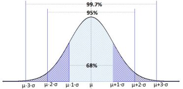
Figure 6-10
For now, we will be working with the most common bell-shaped probability distribution known as the normal distribution, also called the Gaussian distribution, named after the German mathematician Johann Carl Friedrich Gauss. See Figure 6-11.
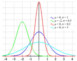
Figure 6-11
A normal distribution is a special type of distribution for a continuous random variable. Normal distributions are important in statistics because many situations in the real world have normal distributions.
Properties of the normal density curve:
- Symmetric bell-shaped.
- Unimodal (one mode).
- Centered at the mean μ= median = mode.
- The total area under the curve is equal to 1 or 100%.
- The spread of a normal distribution is determined by the standard deviation σ. The larger σ is, the more spread out the normal curve is from the mean.
- Follows the Empirical Rule.
If a continuous random variable X has a Normal distribution with mean μ and standard deviation σ then the distribution is denoted as X~N(μ, σ). Any x values from a Normal distribution can be transformed or standardized into a standard Normal distribution by taking the z-score of x.
The formula for the normal probability density function is: . We will not be using this formula.
The probability is found by using integral calculus to find the area under the PDF curve. Prior to the handheld calculators and personal computers, there were probability tables made to look up these areas. This text does not use probability tables and will instead rely on technology to compute the area under the curve.
Every time the mean or standard deviation changes the shape of the normal distribution changes. The center of the normal curve will be the mean and the spread of the normal curve gets wider as the standard deviation gets larger.
Figure 6-12 compares two normal distributions N(0, 1) in green on the left and N(7, 6) in blue on the right.
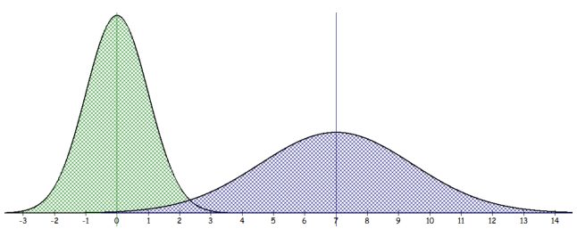
Figure 6-12
“‘So, what's odd about it?’
‘Nothing, it's Perfectly Normal.’”
(Adams, 2002)
6.4.1 Standard Normal Distribution
A normal distribution with mean μ = 0 and standard deviation σ = 1 is called the standard normal distribution.
The letter Z is used exclusively to denote a variable that has a standard normal distribution and is written Z ~ N(0, 1). A particular value of Z is denoted z (lower-case) and is referred to as a z-score.
Recall that a z-score is the number of standard deviations x is from the mean. Anytime you are asked to find a probability of Z use the standard normal distribution.
Standardizing and z-scores:
A z-score is the number of standard deviations an observation x is above or below the mean μ. If the z-score is negative, x is below the mean. If the z-score is positive, x is above the mean.
To find the area under the probability density curve involves calculus so we will need to rely on technology to find the area.
Note that the lower value of the shaded region is -∞, which the TI-84 does not have. Instead we use a really small number in scientific notation -1E99 or -1*1099 (make sure you use the negative sign (-) not the minus – sign.
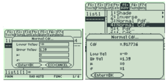
The normalcdf on the calculator needs the lower and upper value of the shaded area followed by the mean and standard deviation. (The TI-89 uses -∞ for the lower boundary instead of -1E99.)
TI-84: Press [2nd] [DISTR] menu, select the normalcdf. Then type in the lower value, upper value, mean = 0, standard deviation = 1 to get normalcdf(-1E99,1.39,0,1) = 0.9177, which is your answer. The area under the curve is equivalent to the probability of getting a z-score less than 1.39, or P(Z < 1.39) = 0.9177.
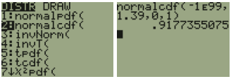
TI-89: Go to the [Apps] Stat/List Editor, then select F5 [DISTR]. This will get you a menu of probability distributions. Arrow down to Normal Cdf and press [ENTER]. Enter the values for the lower z value (z1), upper z value (z2), μ = 0, and σ = 1 into each cell. Press [ENTER]. This is the cumulative distribution function and will return P(z1 < Z < z2). For a left-tail area use a lower bound of negative infinity (-∞), and for a right-tail area use an upper bound infinity (∞).
Excel: For Excel the program will only find the area to the left of a point. Therefore, if we want to find the area to the right of a point or between two points there will be one extra step. Use the formula =NORM.S.DIST(1.39,TRUE).
Using Excel or TI-Calculator to Find Standard Normal Distribution
As you read through a problem look for some of the following key phrases in Figure 6-15. Once you find the phrase then match up to what sign you would use and then use the table to walk you through using Excel or the calculator. Note that we could also use the NORM.DIST function with µ = 0 and σ = 1.
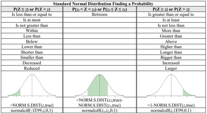
Figure 6-15
6.4.2 Applications of the Normal Distribution
Many variables are nearly normal, but none are exactly normal. Thus, the normal distribution, while not perfect for any single problem, is very useful for a variety of problems. Variables such as SAT scores and heights of United States adults closely follow the normal distribution. Note that the Excel function NORM.S.DIST is for a standard normal when µ = 0 and σ = 1
Using Excel or TI-Calculator to Find Normal Distribution Probabilities
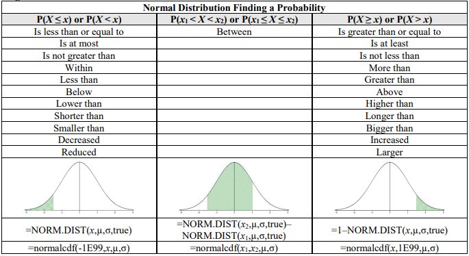
Figure 6-18
TI-84: Press [2nd] [DISTR]. This will show a menu of probability distributions. Arrow down to 2:normalcdf( and press [ENTER]. This puts normalcdf( on the home screen. Enter the values for the lower x value (x1), upper x value (x2), μ, and σ with a comma between each. Press [ENTER]. This is the cumulative distribution function and will return P(x1 < X < x2). For example, to find P(80 < X < 110) when the mean is 100 and the standard deviation is 20, you should have normalcdf(80,110,100,20). If you leave out the μ and σ, then the default is the standard normal distribution. For a left-tail area use a lower bound of –1E99 (negative infinity), (press [2nd] [EE] to get E) and for a right-tail area use an upper bound of 1E99 (infinity). For example, to find P(Z < -1.37) you should have normalcdf(-1E99,-1.37).
TI-89: Go to the [Apps] Stat/List Editor, select F5 [DISTR]. This will show a menu of probability distributions. Arrow down to Normal Cdf and press [ENTER]. Enter the values for the lower x value (x1), upper x value (x2), μ, and σ into each cell. Press [ENTER]. This is the cumulative distribution function and will return P(x1 < X < x2). For example, to find P(80 < X < 110) when the mean is 100 and the standard deviation is 20, you should have in the following order 80, 110, 100, 20. If you have a z-score, use μ = 0 and σ = 1, then you will get a standard normal distribution. For a left-tail area use a lower bound of negative infinity (-∞), and for a right-tail area use an upper bound infinity (∞).
“The Hitchhiker's Guide to the Galaxy offers this definition of the word "Infinite." Infinite: Bigger than the biggest thing ever and then some. Much bigger than that in fact, really amazingly immense, a totally stunning size, "wow, that's big," time. Infinity is just so big that by comparison, bigness itself looks really titchy. Gigantic multiplied by colossal multiplied by staggeringly huge is the sort of concept we're trying to get across here.”
(Adams, 2002)
A nice feature of this section is that the problems will say that the distribution is normally distributed, unlike the discrete distributions where you have to look for certain characteristics. However, when handling real data, you may have to know how to detect whether the data is normally distributed. One way to see if your variable is approximately normally distributed is by looking at a histogram, or we can use a normal probability plot.
6.4.3 Normal Probability Plot
A normal quantile plot, also called a normal probability plot, is a graph that is useful in assessing normality. A normal quantile plot plots the variable x against each of the x values corresponding z-score. It is not practical to make a normal quantile plot by hand.
# Points near the line => approximately normal
set.seed(2)
x <- rnorm(50, 67, 2.5)
qqnorm(x); qqline(x)
Interpreting a normal quantile plot to see if a distribution is approximately normally distributed.
- All of the points should lie roughly on a straight line y = x.
- There should be no S pattern present.
- Outliers appear as points that are far away from the overall pattern of the plot.
Here are two examples of histograms with their corresponding quantile plots. Note that as the distribution becomes closer to a normal distribution the dots on the quantile plot will be in a straighter line. Figures 6-21 is the histogram and figure 6-22 is the corresponding normal probability plot. Note the histogram is skewed to the left and dots do not line up on the y = x line. Figures 6-23 and Figure 6-24 represent a sample that is approximately normally distributed. Note that the dots still do not line up perfectly on the line y = x, but they are close to the line.
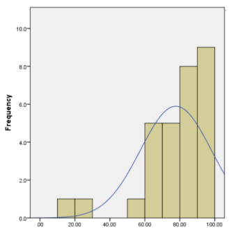
Figure 6-21
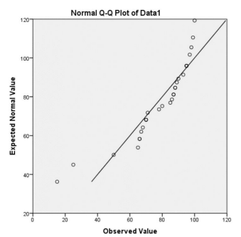
Figure 6-22
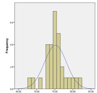
Figure 6-23
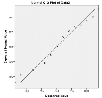
Figure 6-24
6.4.4 Finding Percentiles for a Normal Distribution
Sometimes you will be given an area or probability and have to find the associated random variable x or z-score. For example, the probability below a point on the normal distribution is a percentile. If we find that the P(Z < 1.645) =NORM.S.DIST(1.645,TRUE) = 0.950015, that tells us that about 95% of z-scores are below 1.645. In other words, the z-score of 1.645 is the 95th percentile.
We can use technology to find z-score given a percentile. Most technology has built in commands that will find the probability below a point. If you want to find the area above a point, or between two points, then find the area below a point by using the complement rule and keep in mind that the total area under the curve is 1 and the total area below the mean is 0.5.
If x is an observation from a distribution that has mean μ and standard deviation σ, the standardized value of x (or z-score) is .
TI-84: Press [2nd] [DISTR]. This will get you a menu of probability distributions. Press 3 or arrow down to 3:invNorm( and press [ENTER]. This puts invNorm( on the home screen. Enter the area to the left of the x value, μ, and σ with a comma between each. Press [ENTER]. This will return the percentile for the x value. For example, to find the 95th percentile when the mean is 100 and the standard deviation is 20, you should have invNorm(0.95,100,20). If you leave out the μ and σ, then the default is the z-score for the standard normal distribution
TI-89: Go to the [Apps] Stat/List Editor, then select F5 [DISTR]. This will get you a menu of probability distributions. Arrow down to Inverse Normal and press [ENTER]. Enter the area to the left of the x value, μ, and σ into each cell. Press [ENTER]. This will return the percentile for the x value. For example, to find the 95th percentile when the mean is 100 and the standard deviation is 20, you should enter 0.95, 100, 20.
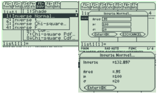
If you use μ = 0 and σ = 1, then the default is the z-score for the standard normal distribution.
Using Excel or TI-Calculator for the Percentile of a Normal Distribution
Note that the NORM.S.INV function is for a standard normal when µ = 0 and σ = 1.
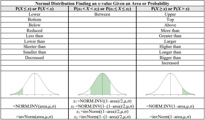
Figure 6-27
Adapted from Mostly Harmless Statistics by Rachel Webb (Portland State University, https://mostlyharmlessstat.wixsite.com/webpage), © Rachel Webb, licensed under CC BY-SA 4.0. Changes were made. License: CC-BY-SA-4.0.