9.1 Two Sample Mean T-Test for Dependent Groups

Dependent samples or matched pairs, occur when the subjects are paired up, or matched in some way. Most often, this model is characterized by selection of a random sample where each member is observed under two different conditions, before/after some experiment, or subjects that are similar (matched) to each other are studied under two different conditions.

There are 3 types of hypothesis tests for comparing two dependent population means µ₁ and µ₂, where, µ_D is the expected difference of the matched pairs.

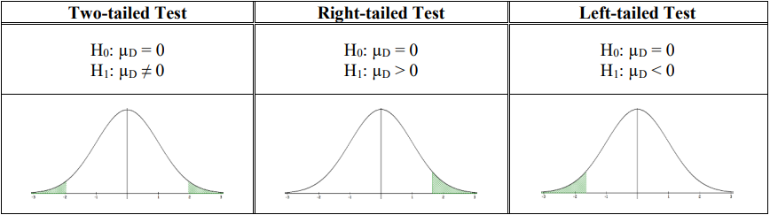
Table of the three hypothesis setups for a paired-means t-test: two-tailed with H0: μD = 0 and H1: μD ≠ 0, right-tailed with H1: μD > 0, and left-tailed with H1: μD < 0, each above a normal curve shaded in both tails, the right tail, or the left tail respectively. — Figure 9-1

Note: If each pair were equal to one another then the mean of the differences would be zero. We could also use this model to test with a magnitude of a difference, but we rarely cover that scenario, therefore we are usually test against the difference of zero.

The t-test for dependent samples is a statistical test for comparing the means from two dependent populations (or the difference between the means from two populations). The t-test is used when the differences are normally distributed. The samples also must be dependent.

Note we will usually only use the case where µ_D equals zero.

The subscript “D” denotes the difference between population one and two. It is important to compute D = x₁ – x₂ for each pair of observations. However, this makes setting up the hypotheses more challenging for one-tailed tests.

If we were looking for an increase in test scores from before to after, then we would expect the after score to be larger. When we take a smaller number minus a larger number then the difference would be negative. If we put the before group first and the after group second then we would need a left-tailed test μ_D < 0 to test the “increase” in test scores. This is opposite of the sign we associate for “increase.” If we swap the order and use the after group first, then the before group would have a larger number minus a smaller number which would be positive and we would do a right-tailed test μ_D > 0.

Always subtract in the same order the data is presented in the question. An easier way to decide on the one-tailed test is to write down the two labels and then put a less than symbol between them depending on the question. For example, if the research statement is a weight loss program significantly decreases the average weight, the sign of the test would change depending on which group came first. If we subtract before weight – after weight, then we would want to have before > after and use μ_D > 0. If we have the after weight as the first measurement then we would subtract the after weight – before weight and want after < before and use μ_D < 0. If you keep your labels in the same order as they appear in the question, compare them and carry this sign down to the alternative hypothesis.

The traditional method (or critical value method), the p-value method, and the confidence interval method are performed with steps that are identical to those when performing hypothesis tests for one population.

Example 1

A dietician is testing to see if a new diet program reduces the average weight. They randomly sample 35 patients and measure them before they start the program and then weigh them again after 2 months on the program. What are the correct hypotheses?

Show solution

Let x₁ = weight before a weight-loss program and x₂ = weight after the weight-loss program. We want to test if, on average, participants lose weight. Therefore, the difference D = x₁ – x₂. This gives D = before weight – after weight, thus if on average people do lose weight, then in general the before > after and the D’s are positive. How we define our differences determines that this example is a right-tailed test (carry the > sign down to the alternative hypothesis) and the correct hypotheses are:

H₀: µ_D = 0

H₁: µ_D > 0

If we were to do the same problem but reverse the order and take D = after weight – before weight the correct alternative hypothesis is H₁: µ_D < 0 since after weight < before weight. Just be consistent throughout your problem, and never switch the order of the groups in a problem.

P-Value Method Example

Example 2

In an effort to increase production of an automobile part, the factory manager decides to play music in the manufacturing area. Eight workers are selected, and the number of items each produced for a specific day is recorded. After one week of music, the same workers are monitored again. The data are given in the table. At $α$ = 0.05, can the manager conclude that the music has increased production? Assume production is normally distributed. Use the p-value method.

Worker

1 2 3 4 5 6 7 8

Before

6 8 10 9 5 12 9 7

After

10 12 9 12 8 13 8 10

Show solution

Assumptions: We are comparing production rates before and after music is played in the manufacturing area. We are given that the production rates are normally distributed. Because these are consecutive times from the same population, they are dependent samples, so we must use the t-test for matched pairs.

Let population 1 be the number of items before the music, and population 2 be after. The claim is that music increases production so before production < after production. Carry this same sign to the alternative hypothesis.

The correct hypotheses are: H₀: µ_D = 0; H₁: µ_D < 0, this is a left-tailed test.

In order to compute the t-test statistic, we must first compute the differences between each of the matched pairs.

Before (x₁)	6	8	10	9	5	12	9	7
After (x₂₎	10	12	9	12	8	13	8	10
D = x₁-x₂	–4	–4	1	–3	–3	–1	1	–3

Using the 1-var stats on the differences in your calculator, we compute $\bar{D} = \bar{x} = - 2$ , s_D = s_x = 2.0702, n = 8.

The test statistic is: $\t equals the fraction D bar minus μ sub D over open parenthesis the fraction s sub D over the square root of n close parenthesis equals the fraction minus 2 minus 0 over open parenthesis the fraction 2.0702 over the square root of 8 close parenthesis equals minus 2.7325$ .

The p-value for a two-tailed t-test with degrees of freedom = n – 1 = 7, is found by finding the area to the left of the test statistic –2.7325 using technology.

Decision: Since the p-value = 0.0146 is less than $α$ = 0.05, we reject H₀.

Summary: At the 5% level of significance, there is enough evidence to support the claim that the mean production rate increases when music is played in the manufacturing area.

TI-84: Find the differences between the sample pairs (you can subtract two lists to do this). Press the [STAT] key and then the [EDIT] function, enter the difference column into list one. Press the [STAT] key, arrow over to the [TESTS] menu. Arrow down to the option [2:T -Test] and press the [ENTER]. Arrow over to the [Data] menu and press the [ENTER] key. Then type in the hypothesized mean as 0, List: L3, leave Freq:1 alone, arrow over to the $\neq$ , <, >, sign that is the same in the problem’s alternative hypothesis statement then press the [ENTER] key, arrow down to [Calculate] and press the [ENTER] key. The calculator returns the t-test statistic, the p-value, mean of the differences $\bar{D} = \bar{x}$ and standard deviation of the differences s_D = s_x.

TI-89: Find the differences between the sample pairs (you can subtract two lists to do this). Go to the [Apps] Stat/List Editor, enter the two data sets in lists 1 and 2. Move the cursor so that it is highlighted on the header of list3. Press [2^nd] Var-Link and move down to list1 and press [Enter]. This brings the name list1 back to the list3 at the bottom, select the minus [-] key, then select [2^nd] Var-link and this time highlight list2 and press [Enter]. You should now see list1-list2 at the bottom of the window. Press [Enter] then the differences will be stored in list3. Press [2^nd] then F6 [Tests], select 2: T-Test. Select the [Data] menu. Then type in the hypothesized mean as 0, List: list1, Freq:1, arrow over to the $\neq$ , <, >, and select the sign that is the same in the problem’s alternative hypothesis, press the [ENTER] key to calculate. The calculator returns the t-test statistic, p-value, $\bar{D} = \bar{x}$ and s_D = s_x.

Excel: Start by entering the data in two columns in the same order that they appear in the problem. Then select Data > Data Analysis > t-test: Paired Two Sample for Means, then select OK.

Select the Before data (including the label) into the Variable 1 Range, and the After data (including the label) in the Variable 2 Range. Type in zero for the Hypothesized Mean Difference box. Select the box for Labels (do not select this if you do not have labels in the variable range selected). Change alpha to fit the problem. You can leave the default to open in a new worksheet or change output range to be one cell where you want the top left of the output table to start (make sure this cell does not overlap any existing data). Then select OK. See below for example.

You get the following output:

One nice feature in Excel is that you get the p-value and the critical value in the output. The critical value can be taken from the Excel output; however, Excel never gives negative critical values. Since we are doing a left-tailed test we will need to use the t-score = -1.8946.

If we were to draw and shade the critical region for the sampling distribution, it would look like Figure 9 -2.

Figure 9-2

The decision is made by comparing the test statistic t = -2.7325 with the critical value t_α = -1.8946.

Since the test statistic is in the shaded critical region, we would reject H₀.

At the 5% level of significance, there is enough evidence to support the claim that the mean production rate increases when music is played in the manufacturing area.

The decision and summary should not change from using the p-value method.

Confidence Interval Method

Example 3

Hands-On Café records the number of online orders for eight randomly selected locations for two consecutive days. Assume the number of online orders is normally distributed. Find the 95% confidence interval for the mean difference. Is there evidence of a difference in mean number of orders for the two days?

Location

1 2 3 4 5 6 7 8

Thursday

67 65 68 68 68 70 69 70

Friday

68 70 69 71 72 69 70 70

Show solution

First set up the hypotheses. We are testing to see if Thursday $\neq$ Friday orders. The hypotheses would be:

H₀: µ_D = 0

H₁: µ_D ≠ 0

Next, compute the \(\frac{t_

ParseError: invalid DekiScript

(click for details)

Callstack: at (Bookshelves/Introductory_Statistics/Mostly_Harmless_Statistics_(Webb)/09:_Hypothesis_Tests_and_Confidence_Intervals_for_Two_Populations/9.01:_Two_Sample_Mean_T-Test_for_Dependent_Groups), /content/body/section[5]/div/table/div/p[4]/span, line 1, column 1

\) critical value for a 95% confidence interval and df = 7. Use the t-distribution with technology using confidence level 95%, lower tail area of $α$ /2 = 0.025 to get t

$α$ /2

= t

0.025

= ±2.36462. Compute the differences of Thursday – Friday for each pair.

Thursday	67	65	68	68	68	70	69	70
Friday	68	70	69	71	72	69	70	70
D	–1	–5	–1	–3	–4	1	–1	0

Use technology to compute the mean, standard deviation and sample size.

Note if you use a TI calculator then $\bar{D} = \bar{x}$ and s_D = s_x.

Find the interval estimate: $\bar{D} \pm t_{\frac{α}{2}} (\frac{s_{D}}{\sqrt{n}})$

$\begin{aligned}
&\Rightarrow-1.75 \pm 2.36462\left(\frac{2.05287}{\sqrt{8}}\right) \\
&\Rightarrow-1.75 \pm 1.7162.
\end{aligned}$

Write the answer using standard notation –3.4662 < μ_D < –0.0335 or interval notation (–3.4662, –0.0338).

For an interpretation of the interval, if we were to use the same sampling techniques, approximately 95 out of 100 times the confidence interval (–3.4662, –0.0338) would contain the population mean difference in the number of orders between Thursday and Friday.

Since both endpoints are negative, we can be 95% confident that the population mean number of orders for Thursday is between 3.4662 and 0.0338 orders lower than Friday.

Excel: Type in both samples in two adjacent columns, and then subtract each pair in a third column and label the column Difference.

Thursday	Friday	Difference
67	68	=A2-B2
65	70	=A3-B3
68	69	=A4-B4
68	71	=A5-B5
68	72	=A6-B6
70	69	=A7-B7
69	70	=A8-B8
70	70	=A9-B9

Select Data > Data Analysis > Descriptive Statistics and click OK.

Select the Difference column for the input range including the label, then check the box next to Labels in first row (do not select this box if you did not highlight a label in the input range). Use the default new worksheet or select a single cell for the Output Range where you want your top left-hand corner of the table to start. Check the boxes Summary Statistics and Confidence Level for Mean. Change the confidence level to fit the question, and then select OK.

You get the following output:

The confidence interval is the mean ± margin of error. In two different cells subtract and then add the margin of error from the mean to get the confidence interval limits and then put your answer in interval notation (–3.4662, – 0.0338).

TI-84: First, find the differences between the samples. Then on the TI-83 press the [STAT] key, arrow over to the [TESTS] menu, arrow down to the [8:TInterval] option and press the [ENTER] key. Arrow over to the [Data] menu and press the [ENTER] key. The defaults are List: L1, Freq:1. If this is set with a different list, arrow down and use [2^nd] [1] to get L1. Then type in the confidence level. Arrow down to [Calculate] and press the [ENTER] key. The calculator returns the confidence interval, $\bar{D} = \bar{x}$ and s_D = s_x.

TI-89: First, find the differences between the samples. Go to the [Apps] Stat/List Editor, then enter the differences into list 1. Press [2^nd] then F7 [Ints], then select 2: T-Interval. Select the [Data] menu. Enter in List: list1, Freq:1. Then type in the confidence level. Press the [ENTER] key to calculate. The calculator returns the confidence interval, $\bar{D} = \bar{x}$ and s_D = s_x.

Adapted from Mostly Harmless Statistics by Rachel Webb (Portland State University), hosted on LibreTexts (stats.libretexts.org) and licensed under CC BY-SA 4.0. Changes were made. License: CC-BY-SA-4.0.