12.11 Multiple Linear Regression

A multiple linear regression line describes how two or more predictor variables affect the response variable $y$ . An equation of a line relating $p$ independent variables to $y$ is of the form for the population as: $y = β_{0} + β_{1} x_{1} + β_{2} x_{2} + \dots + β_{p} x_{p} + ε$ , where $β sub 1, β sub 2, …, β sub p$ are the slopes, $β sub 0$ is the $y$ -intercept and $ε$ is called the error term.

We use sample data to estimate this equation using the predicted value of $y$ as $\hat{y}$ with the regression equation (also called the line of best fit or least squares regression line) as:

$y = b_{0} + b_{1} x_{1} + b_{2} x_{2} + \dots + b_{p} x_{p}$

where $b sub 1, b sub 2, …, b sub p$ are the slopes, and $b sub 0$ is the $y$ -intercept

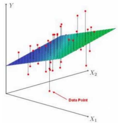
For example, if we had two independent variables, we would have a 3-dimensional space as in Figure 12-25 where the red dots represent the sample data points and the equation would be a plane in the space represented by $y = b_{0} + b_{1} x_{1} + b_{2} x_{2}$ .

A three-dimensional coordinate system with axes for x1 and x2 forming the "floor" and the y-axis running vertically, containing a number of data points in red. A diagonal plane represents the "best fit" of these data points, with a vertical line connecting each point to the plane. — Figure 12-25: Multiple linear regression with 2 independent variables. This photo by unknown author is licensed under CC BY-SA-NC.

The calculations use matrix algebra, which is not a prerequisite for this course. We will instead rely on a computer to calculate the multiple regression model.

If all the population slopes were equal to zero, the model $y = β_{0} + β_{1} x_{1} + β_{2} x_{2} + \dots + β_{p} x_{p} + ε$ would not be significant and should not be used for prediction. If one or more of the population slopes are not equal to zero then the model will be significant, meaning there is a significant relationship between the independent variables and the dependent variable and we may want to use this model for prediction. There are other statistics to look at to decide if this would be the best model to use. Those methods are discussed in more advanced courses.

The hypotheses will always have an equal sign in the null hypotheses.

The hypotheses are:

$H_{0} : β_{1} = β_{2} = \dots = β_{p} = 0$
$H sub 1:$ At least one slope is not zero.

Note that the alternative hypothesis is not written as $H sub 1: β sub 1 not equal to β sub 2 not equal to ⋯ not equal to β sub p not equal to 0$ . This is because we just want one or more of the independent variables to be significantly different from zero, not necessarily all the slopes unequal to zero.

Use the F-distribution with degrees of freedom for regression = $d f_{R} = p$ , where $p$ = the number of independent variables (predictors), and degrees of freedom for error = $d f_{E} = n - p - 1$ , where $n$ is the number of pairs. This is always a right-tailed ANOVA test, since we are testing if the variation in the regression model is larger than the variation in the error.

The test statistic and p-value are the last two values on the right in the ANOVA table. The p-value rule is easiest to use since the p-value is part of the outcome, but a critical value can be found using the invF program on your calculator or in Excel using =F.INV.RT( $α, d f_{R}, d f_{E}$ ) We can also single out one independent variable at a time and use a t-test to see if the variable is significant by itself in predicting $y$ .

This would have hypotheses:

$H sub 0: β sub i equals 0$
$H sub 1: β sub i not equal to 0$
where $i$ is a placeholder for whichever independent variable is being tested.

This t-test is found in the same row as the coefficient that you are testing.

Assumptions for Multiple Linear Regression

When doing multiple regression, the following assumptions need to be met:

The residuals of the model are approximately normally distributed.
The residuals of the model are independent (not autocorrelated) and have a constant variance (homoscedasticity).
There is a liner relationship between the dependent variable and each independent variable.
Independent variables are uncorrelated with each other (no multicollinearity).

The following is a schematic for the regression output for Microsoft Excel. Other software usually has a similar output but may have numbers in slightly different places. The blue spaces have the descriptions of the corresponding numbers.

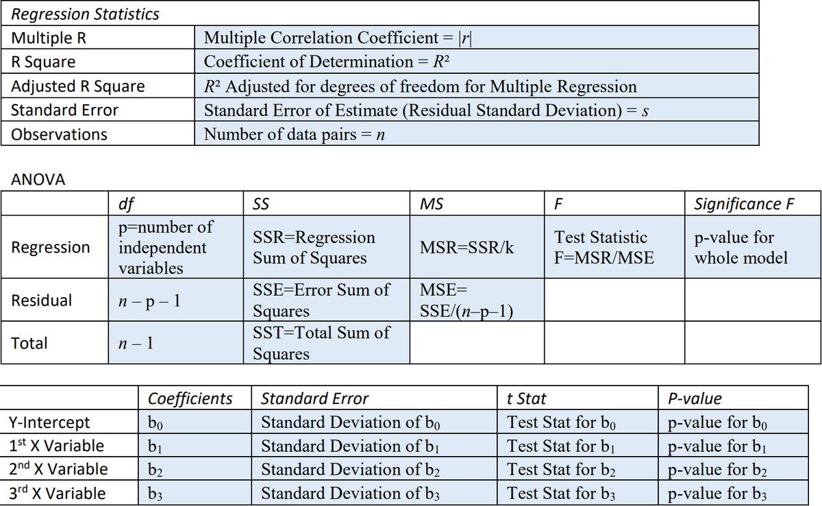
Excel-generated regression statistics table, ANOVA table, and table of coefficients, standard error, t-stat and p-value for the y-intercept, first x variable, second x variable, and third x variable. — Figure 12-26: Excel output for multiple linear regression.

The coefficients column gives the numeric values to find the regression equation $y = b_{0} + b_{1} x_{1} + b_{2} x_{2} + \dots + b_{p} x_{p}$ . The p-values for $b_{i}$ should be investigated to see if the variable is statistically significant. One should also be careful that the independent variables are not significantly correlated amongst themselves. Correlated independent variables may give unexpected outcomes in the overall regression model and actually flip the sign on a coefficient.

Example 1

A sample of 30 homes that were recently on the market were selected. The listing price in $1,000’s of the home, the livable square feet of the home, the lot size in 1,000’s of square feet and the number of bathrooms in the home were recorded. A multiple linear regression was done in Excel with the following output. Test to see if there is a significant relationship between the listing price of a home with the livable square feet, lot size, and number of bathrooms. If there is a relationship, then use the regression model to predict the listing price for a home that has 2,350 square feet, 3 bathrooms and has a 5,000 square foot lot. Use $α$ = 0.05.

Show solution

First, we need to test to see if the overall model is significant.

The hypotheses are:

$H_{0} : β_{1} = β_{2} = β_{3} = 0$
$H sub 1:$ At least one slope is not zero.

The test statistic is $F equals 187.9217$ and the p-value = $9.74 E minus 18 ~ 0$

We reject $H sub 0$ , since the p-value is less than $α$ = 0.05. There is enough evidence to support the claim that there is a significant relationship between the number of bathrooms and lot size of a home with its listing price. Since we reject $H sub 0$ , we can use the regression model for prediction.

The question asked to predict the listing price for a home that has 2,350 square feet, 3 bathrooms and has a 5,000 square foot lot. This gives us $x sub 1 equals 2350$ , $x sub 2 equals 5$ (5,000 square feet), and $x sub 3 equals 3$ .

The coefficients column has the values that correspond to the y-intercept and slopes gives the regression equation: $\hat{y} = - 28.8477 + 0.170908 \cdot x_{1} + 6.7705 \cdot x_{2} + 15.5347 \cdot x_{3}$ .

Substitute the three given x values into the equation in the correct order and you get $\hat{y} = - 28.8477 + 0.170908 \cdot 2350 + 6.7705 \cdot 5 + 15.5347 \cdot 3 = 453.2787$ .

This then gives a predicted listing price of $453,278.

Note that our sample size is very small and we really need to check assumptions in order to use this predicted value with any reliability.

Is this the best model to use? Note that not all the p-values for each of the individual slope coefficients are significant. The number of bathrooms has a t-test statistic = 1.687038 and p-value = 0.10356, which is not statistically significant at the 5% level of significance.

We may want to rerun the regression model without the number of bathroom variables and see if we get a higher $R^{2}$ and a lower standard error of estimate. Ideally, we would try all the different combinations of independent variables and see which combination gives the best model. This is a lot of work to do if you have many independent variables. Most statistical software packages have built in functions that find the best fit.

Adjusted Coefficient of Determination

When we add more predictor variables into the model, this inflates the coefficient of variation, $R^{2}$ . In multiple regression, we adjust for this inflation using the following formula for adjusted coefficient of variation.

Adjusted Coefficient of Determination

$R_{a d j}^{2} = 1 - (\frac{(1 - R^{2}) (n - 1)}{(n - p - 1)})$

There are more types of regression models and more that should be done for a complete regression analysis. Ideally, you would find several models and pick the one with no outliers, the smallest standard error of estimate, a good residual plot, and the highest adjusted $R^{2}$ and check the assumptions behind each model before using for prediction. More advanced techniques are discussed in a regression course.

“Well, I was in fact, I was moving backwards in time. Hmmm. Well, I think we've sorted all that out now. If you'd like to know, I can tell you that in your universe you move freely in three dimensions that you call space. You move in a straight line in a fourth, which you call time, and stay rooted to one place in a fifth, which is the first fundamental of probability. After that it gets a bit complicated, and there's all sorts of stuff going on in dimensions 13 to 22 that you really wouldn't want to know about. All you really need to know for the moment is that the universe is a lot more complicated than you might think…”

(Adams, 2002)

Adapted from Mostly Harmless Statistics by Rachel Webb (Portland State University), hosted on LibreTexts (stats.libretexts.org) and licensed under CC BY-SA 4.0. Changes were made. License: CC-BY-SA-4.0.