5.4 Binomial Distribution

The binomial distribution is a discrete probability distribution used to find the probability of success when there are two outcomes to each trial, and there are a set number of independent trials with the same probability of occurrence. To develop the process for calculating the probabilities in a binomial experiment, consider the following example.

Example 1

Suppose you are given a three-question multiple-choice test. Each question has four responses and only one is correct. Suppose you want to find the probability that you can just guess at the answers and get two questions correct. To help with the idea that you are going to guess, suppose the test is on string theory.

Is this a binomial experiment? Since all of the properties are met, this is a binomial experiment.
What is the probability of getting two questions right?
What is the probability of getting zero right, one right, two right and all three right?

Show solution

a) The random variable is x = number of correct answers. 1. There are three questions, and each question is a trial, so there are a fixed number of trials. In this case, n = 3. 2. Getting the first question right has no effect on getting the second or third question correct, thus the trials are independent. 3. Either you get the question right or you get it wrong, so there are only two outcomes. In this case, the success is getting the question right. 4. The probability of getting a question right is one out of four. This is the same for every trial since each question has 4 responses. In this case, p = ¼ and q = 1 – ¼ = ¾.

b) To answer this question, start with the sample space. SS = {RRR, RRW, RWR, WRR, WWR, WRW, RWW, WWW}, where RRW means you get the first question right, the second question right, and the third question wrong.

Now the event space for getting 2 right is {RRW, RWR, WRR}. What you did in chapter four was just to find three divided by eight to compute the probability outcome. However, this would not be correct in this case, because the probability of getting a question right is different from getting a question wrong. What else can you do?

Look at just P(RRW) for the moment. Again, that means P(RRW) = P(R on 1st, R on 2nd, and W on 3rd). Since the trials are independent, then P(RRW) = P(R on 1st, R on 2nd, and W on 3rd) = P(R on 1st) * P(R on 2nd) * P(W on 3rd). Just multiply p · p · q = P(RRW) = ¼ ∙ ¼ ∙ ¾ = (¼)² ∙ (¾)¹.

Similarly, you can compute the P(RWR) and P(WRR). To find the probability of 2 correct answers, just add these three probabilities together.

P(2 correct answers) = P(RRW) + P(RWR) + P(WRR) = (¼)² ∙ (¾)¹ + (¼)² ∙ (¾)1 + (¼)² ∙ (¾)¹ = 3∙(¼)² ∙ (¾)¹.

c) You could go through the same argument that you did above and come up with the following:

Do you see the resulting pattern? You can now write the general formula for the probabilities for a binomial experiment.

First, the random variable in a binomial experiment is x = number of successes.

A binomial probability distribution results from a random experiment that meets all of the following requirements.

The procedure has a fixed number of trials (or steps), which is denoted by n.
The trials must be independent.
Each trial must have exactly two categories that can be labeled “success” and “failure.”
The probability of a “success,” denoted by p, remains the same in all trials. The probability of “failure” is often denoted by q, thus q = 1 – p.
Random Variable, X, counts the number of “successes.”

If a random experiment satisfies all of the above, the distribution of the random variable X, where X counts the number of successes, is called a binomial distribution. A binomial distribution is described by the population proportion p and the sample size n. If a discrete random variable X has a binomial distribution with population proportion p and sample size n, we write X ~ B(n, p).

Be careful, a “success” is not always a “good” thing. Sometimes a success is something that is “bad,” like finding a defect or getting in a car crash. The success will be the event from the probability question.

The geometric and binomial distributions are easy to mix up. Keep in mind that the binomial distribution has a given sample size, whereas the geometric is sampling until you get a success.

Excel Formula for Binomial Distribution: For exactly P(X = x) use =binom.dist(x,n,p,false).

For P(X ≤ x) use =binom.dist(x,n,p,true).

TI-84: Press [2nd] [DISTR]. This will get you a menu of probability distributions. Press 0 or arrow down to 0:binompdf( and press [ENTER]. This puts binompdf( on the home screen. Enter the values for n, p and x with a comma between each. Press [ENTER]. This is the probability density function and will return you the probability of exactly x successes. If you leave off the x value and just enter n and p, you will get all the probabilities for each x from 0 to n. Press [ALPHA] A or arrow down to A:binomcdf( and press [ENTER]. This puts binomcdf( on the home screen. Enter the values for n, p and x with a comma between each. If you have the newer operating system on the TI84, the screen will prompt you for each value. Press [ENTER]. This is the cumulative distribution function and will return you the probability of at most (≤) x successes. If you have at least x success (≥), use the complement rule. If you have < or > adjust x to get ≤ or ≥.

TI-89: Go to the [Apps] Stat/List Editor, then select F5 [DISTR]. This will get you a menu of probability distributions. Arrow down to binomial Pdf and press [ENTER]. Enter the values for n, p and x into each cell. Press [ENTER]. This is the probability density function and will return you the probability of exactly x successes. If you leave off the x value and just enter n and p, you will get all the probabilities for each x from 0 to n. Arrow down to binomial Cdf and press [ENTER]. Enter the values for n, p and lower and upper value of x into each cell. Press [ENTER]. This is the cumulative distribution function and will return you the probability between the lower and upper x-values, inclusive.

Example 2

When looking at a person’s eye color, it turns out that only 2% of people in the world have green eyes (not to be confused with hazel colored eyes). Consider a randomly selected group of 20 people.

Is this a binomial experiment?
Compute the probability that none have green eyes.
Compute the probability that nine have green eyes.

Show solution

a) Yes, since all the requirements are met:

There are 20 people, and each person is a trial, so there are a fixed number of trials.
If you assume that each person in the group is chosen at random the eye color of one person does not affect the eye color of the next person, thus the trials are independent.
Either a person has green eyes or they do not have green eyes, so there are only two outcomes. In this case, the success is a person has green eyes.
The probability of a person having green eyes is 0.02. This is the same for every trial since each person has the same chance of having green eyes.

b) You are looking for P(X = 0), since this problem is asking for none x = 0. There are 20 people so n = 20. The success is selecting someone with green eyes, so the probability of a success p = 0.02. Then the probability of not selecting someone with green eyes is q = 1 – p = 1 – 0.02 = 0.98. Using the formula: P(X = 0) = ₂₀C₀· 0.02⁰ · 0.98^(20-0) = 0.6676. Thus, there is a 66.76% chance that in a group of 20 people none of them will have green eyes.

c) P(X = 9) = binom.dist(9,20,0.02,false) = 6.8859E-11 = 0.00000000006859 which is zero rounded to four decimal places. The probability that out of 20 people, nine of them have green eyes is a very small chance and would be considered a rare event.

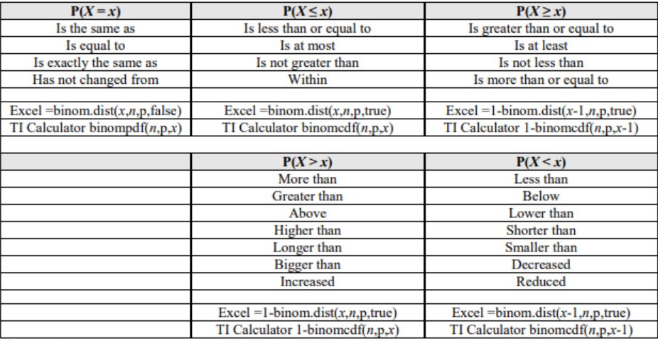
As you read through a problem look for some of the following key phrases in Figure 5-6. Once you find the phrase then match up to what sign you would use and then use the table to walk you through the computer or calculator formula. The same idea about signs applies to all the discrete probabilities that follow.

Table matching probability phrases such as is at most, is at least, more than, and less than to binomial formulas: P(X = x) uses Excel =binom.dist(x,n,p,false) and TI binompdf(n,p,x); P(X ≤ x) uses =binom.dist(x,n,p,true) and binomcdf(n,p,x); P(X ≥ x) uses =1-binom.dist(x-1,n,p,true) and 1-binomcdf(n,p,x-1); P(X > x) uses =1-binom.dist(x,n,p,true) and 1-binomcdf(n,p,x); P(X < x) uses =binom.dist(x-1,n,p,true) and binomcdf(n,p,x-1).

Figure 5-6

Example 3

As of 2018, the Centers for Disease Control and Prevention (CDC) reported that about 1 in 88 children in the United States have been diagnosed with autism spectrum disorder (ASD). A researcher randomly selects 10 children. Compute the probability that 2 children have been diagnosed with ASD.

Show solution

The random variable x = number of children with ASD. There are 10 children, and each child is a trial, so there are a fixed number of trials. In this case, n = 10. If you assume that each child in the group is chosen at random, then whether a child has ASD does not affect the chance that the next child has ASD. Thus, the trials are independent. Either a child has been diagnosed with ASD or they have not been diagnosed ASD, so there are two outcomes. In this case, the success is a child has ASD. The probability of a child having ASD is 1/88. This is the same for every trial since each child has the same chance of having ASD, $p = \frac{1}{88} and q = 1 - \frac{1}{88} = \frac{87}{88}$

Using the formula: $P (X = 2) =_{10} C_{2} \cdot {(\frac{1}{88})}^{2} \cdot {(\frac{87}{88})}^{(10 - 2)} = 0.0053$

Using the TI-83/84 Calculator: P(X = 2) = binompdf(10,1/88,2) = 0.0053.

Using Excel: =BINOM.DIST(2,10,1/88,FALSE) = 0.0053.

Example 4

Flip a fair coin exactly 10 times.

a) What is the probability of getting exactly 8 tails?

b) What is the probability of getting 8 or more tails?

Show solution

a) There are only two outcomes to each trial, heads or tails. The coin flips are independent and the probability of a success, flipping a tail, p = ½ = 0.5 is the same for each trial. This is a binomial experiment with a sample size n = 10. Using the formula: P(X = 8) = ₁₀C₈·0.58 ·0.5^(10-8) = 0.0439

b) We still have p = 0.5 and n = 10, however we need to look at the probability of 8 or more. The P(X ≥ 8) = P(X = 8) + P(X =9) + P(X = 10). We can stop at x = 10 since the coin was only flipped 10 times. P(X ≥ 8) = ₁₀C₈· 0.58 · 0.5^(10-8) + ₁₀C₉· 0.59 · 0.5^(10-9) + ₁₀C₁₀· 0.5¹⁰· 0.5^(10-10) = 0.0439 + 0.0098 + 0.0010 = 0.0547.

So far, most of the examples for the binomial distribution were for exactly x successes. If we want to find the probability of accumulation of x values then we would use the cumulative distribution function (cdf) instead of the pdf. Phrases such as “at least,” “more than,” or “below” can drastically change the probability answers.

Example 5

Approximately 10.3% of American high school students drop out of school before graduation. Choose 10 students entering high school at random. Find the following probabilities.

a) No more than two drop out.

b) At least 6 students graduate.

c) Exactly 10 stay in school and graduate.

Show solution

a) There is a set sample size of independent trials. The person either has or has not dropped out of school before graduation. A “success” is what we are finding the probability for, so in this case a success is to drop out so p = 0.103 and q = 1 – 0.103 = 0.897.

P(X ≤ 2) = P(X = 0) + P(X = 1) + P(X = 2) = ₁₀C₀ · 0.103⁰ · 0.897¹⁰ + ₁₀C₁ · 0.103¹ ·0.897⁹ + ₁₀C₂ · 0.103² · 0.897⁸ = 0.3372 + 0.3872 + 0.2001 = 0.9245

Calculator shortcut use binompdf(10,0.103,0) + binompdf(10,0.103,1) + binompdf(10,0.103,2) = 0.9245 or the binomcdf(10,0.103,2) = 0.9245. On the TI-89 cdf enter the lower value of x as 0 and upper value of x as 2.

In Excel use the function =BINOM.DIST(2,10,0.103,TRUE). Note that if you choose False under cumulative this would return just the P(X = 2) not P(X ≤ 2).

b) A success is to graduate so p = 0.897 and q = 0.103.

P(X ≥ 6) = P(X = 6) + P(X = 7) + P(X = 8) + P(X = 9) + P(X = 10) = ₁₀C₆· 0.897⁶ · 0.103⁴ + ₁₀C₇ · 0.897⁷ · 0.103³ + ₁₀C₈ · 0.897⁸ · 0.103² + ₁₀C₉ · 0.897⁹ · 0.103¹ + ₁₀C₁₀ · 0.897¹⁰ · 0.103⁰ = 0.0123 + 0.0613 + 0.2001 + 0.3872 + 0.3372 = 0.9981.

This is a lot of work to do each one so we can use technology to find the answer.

Note that Excel and the older TI-84 programs only find the probability below x so you have to use the complement rule.

For the TI-84 calculator shortcut use binompdf(10,0.897,6) + binompdf(10,0.897,7) + binompdf(10,0.897,8) + binompdf(10,0.897,9) + binompdf(10,0.897,10) = 0.9981 or use the complement rule P(X ≥ 6) = 1– P(X≤5) = 1–binomcdf(10,0.897,5) = 0.9981.

On the TI-89, just use the binomcdf with the lower x value as 6 and the upper x value as 10.

In Excel use =1–BINOM.DIST(5,10,0.897,TRUE).

c) A success is to graduate so p = 0.897 and q = 0.103. Find P(X = 10) = ₁₀C₁₀· 0.897¹⁰· 0.103⁰ = 0.3372.

On the TI-84 use binompdf(10,0.897,10) = 0.3372.

In Excel =BINOM.DIST(10,10,0.897,FALSE) = 0.3372.

Example 6

When looking at a person’s eye color, it turns out that only 2% of people in the world have green eyes (not to be confused with hazel colored eyes). Consider a randomly selected group of 20 people.

a) Compute the probability that at most 3 have green eyes.

b) Compute the probability that less than 3 have green eyes.

c) Compute the probability that more than 3 have green eyes.

d) Compute the probability that 3 or more have green eyes.

Show solution

a) This fits a binomial experiment. P(X ≤ 3) = P(X = 0) + P(X = 1) + P(X = 2) + P(X = 3) = ₂₀C₀ · 0.02⁰ · 0.80²⁰ + ₂₀C₁ · 0.02¹ · 0.80¹⁹ + ₂₀C₂ · 0.02² · 0.80¹⁸ + ₂₀C₃ · 0.023 · 0.80¹⁷ = 0.667608 + 0.272493 + 0.05283 + 0.006469 = 0.9994.

On the TI-84 use binomcdf(20,0.02,3) = 0.9994.

In Excel =BINOM.DIST(3,20,0.02,true) = 0.9994.

b) P(X < 3) = P(X = 0) + P(X = 1) + P(X = 2) = 0.667608 + 0.272493 + 0.05283 = 0.9929.

On the TI-84 use binomcdf(20,0.02,2) = 0.9929.

In Excel =BINOM.DIST(2,20,0.02,true) = 0.9929.

c) P(X > 3) = 1 – P(X ≤ 3) = 1 – 0.9994 = 0.0006.

On the TI-84 use 1-binomcdf(20,0.02,3) = 0.0006.

In Excel =1-BINOM.DIST(3,20,0.02,true) = 0.0006.

d) P(X ≥ 3) = 1 – P(X ≤ 2) = 1 – 0.9929 = 0.0071

On the TI-84 use 1-binomcdf(20,0.02,2) = 0.0071.

In Excel =1-BINOM.DIST(2,20,0.02,true) = 0.0071.

Example 7

Show solution

$P (X \geq 2) = 1 - P (X \leq 1) = 1 - (_{10} C_{0} \cdot {(\frac{1}{88})}^{0} \cdot {(\frac{87}{88})}^{10 - 0)} +_{10} C_{1} \cdot {(\frac{1}{88})}^{1} \cdot {(\frac{87}{88})}^{(10 - 1)}) = 1 - (0.89202 + 0.102528) = 0.0055$

On the TI-84 use 1-binomcdf(10,1/88,1) = 0.0055.

In Excel =1-BINOM.DIST(1,10,1/88,true) = 0.0055.

Mean, Variance & Standard Deviation of a Binomial Distribution

If you list all possible values of x in a Binomial distribution, you get the Binomial Probability Distribution (pdf). You can then find the mean, the variance, and the standard deviation using the general formulas μ = Σ(x_i ∙ P(x_i)) and σ² = ∑(x_i² ∙P(x_i)) – μ². This, however, would take a lot of work if you had a large value for n. If you know the type of distribution, like binomial, then you can find the mean, variance and standard deviation using easier formulas. They are derived from the general formulas. For a Binomial distribution, μ, the expected number of successes, σ², the variance, and σ, the standard deviation for the number of success are given by the formulas, where p is the probability of success and q = 1 – p.

Example 9

When looking at a person’s eye color, it turns out that only 2% of people in the world have green eyes (not to be confused with hazel colored eyes). Consider a randomly selected group of 20 people. Compute the mean, variance and standard deviation.

Show solution

Since this is a binomial experiment, then you can use the formula μ = n ∙ p. So μ = 20 · 0.02 = 0.4 people. You would expect on average that out of 20 people, less than 1 would have green eyes. The variance would be σ² = n ∙ p ∙ q = 20(0.02)(0.98) = 0.392 people². Once you have the variance, you just take the square root of the variance to find the standard deviation σ = $the square root of 0.392$ = 0.6261 people. We would expect on average spread of the distribution to have 0.4 $\pm$ 0.6261 or 0 to 1 person out of 20 people to have green eyes.

Adapted from Mostly Harmless Statistics by Rachel Webb (Portland State University), hosted on LibreTexts (stats.libretexts.org) and licensed under CC BY-SA 4.0. Changes were made. License: CC-BY-SA-4.0.