5.2 Discrete Probability Distributions

In many cases, the random variable is what you are measuring, but when it comes to discrete random variables, it is usually what you are counting. For the example of height, the random variable is the height of the child. For the example of how many fleas are on prairie dogs in a colony, the random variable is the number of fleas on a prairie dog in a colony.

Now suppose you put all the possible values of the random variable together with the probability that the random variable would occur. You could then have a distribution like before, but now it is called a probability distribution since it involves probabilities. A probability distribution is an assignment of probabilities to all the possible values of the random variable. The abbreviation of pdf is used for a probability density (distribution) function in your calculators.

The probability distribution of X lists all the possible values of x and their corresponding probabilities.

Example 2

A random experiment consists of flipping a fair coin three times. Let X = the number of heads that show up. Create the probability distribution of X.

Show solution

When you flip a coin three times, you can get 0 heads, 1 head, 2 heads or 3 heads, the corresponding values of x are 0, 1, 2, 3. We can find the probabilities for each of these values by finding the sample space and using the classical method of computing probability.

The sample space is S = {HHH, HHT, HTH, THH, HTT, THT, TTH, TTT}.

The event x = 0 can happen one way, namely {TTT}. Thus P(X = x) = P(X = 0) = $\frac{1}{8}$ .

The event x = 1 can happen three ways, namely {HTT, THT, TTH}. Thus P(X = 1) = $\frac{3}{8}$ .

The event x = 2 can happen three ways, namely {HHT, HTH, THH}. Thus P(X = 2) = $\frac{3}{8}$ .

The event x = 3 can happen one way, namely {HHH}. Thus P(X = 3) = $\frac{1}{8}$ .

Therefore, the probability distribution of X is:

x 0 1 2 3 P(X=x) $\frac{1}{8}$ $\frac{3}{8}$ $\frac{3}{8}$ $\frac{1}{8}$

Figure 5-1

Note this is a valid probability distribution because the probability of each x, P(x), is between 0 and 1, and the probability of the sum of all x values from 0 to 3 is ∑ P (x) = $\frac{1}{8} + \frac{3}{8} + \frac{3}{8} + \frac{1}{8} = 1$ .

Figure 5-2 is a graph of the probability distribution using Example 5-2.

Figure 5-2

The height of each line corresponds to the probability of each x value. Sometimes you will see a bar graph instead.

Example 3

The following table shows the probability of winning an online video game, where X = the net dollar winnings for the video game. Is the following table a valid discrete probability distribution?

x -5 -2.5 0 2.5 5 P(X=x) 0.55 $\frac{1}{4}$ 0.15 0 5%

Show solution

It is easier to have all the probabilities as proportions: ¼ = 0.25 and 5% = 0.05. Each probability is a number between 0 and 1: 0 ≤ 0.55 ≤ 1, 0 ≤ 0.25 ≤ 1, 0 ≤ 0.15 ≤ 1, 0 ≤ 0 ≤ 1, 0 ≤ 0.05 ≤ 1. The sum of the probabilities is equal to one: is Σ P(x) = 0.55 + 0.25 + 0.15 + 0 + 0.05 = 1. Yes, this is a valid discrete probability distribution since the table has the two properties that each probability is between 0 and 1, and the sum of the probabilities is one.

Words Are Important!

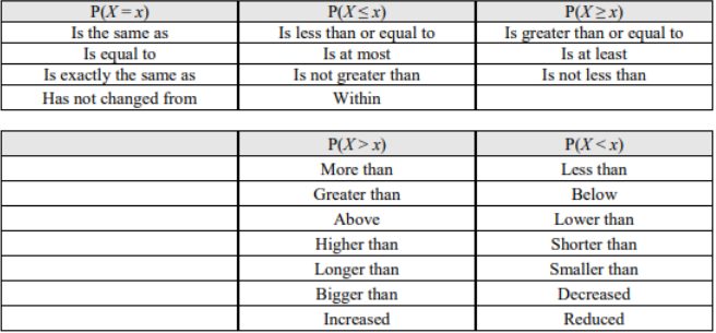
When finding probabilities pay close attention to the following phrases.

Figure 5-2

Example 5

The following is a valid discrete probability distribution of X = the net dollar winnings for an online video game. Find the probability of winning at most $2.50.

x -5 -2.5 0 2.5 5 P(X=x) 0.55 $\frac{1}{4}$ 0.15 0 5%

Show solution

It is easier to have all the probabilities as proportions: ¼ = 0.25 and 5% = 0.05.

At most means the same as, less than or equal to. The probabilities can be found by adding all the probabilities that are less than or equal to 2.5. P(X ≤ 2.5) = 0.55 + 0.25 + 0.15 + 0 = 0.95.

You can also use the complement rule since all the probabilities add to one.

P(X ≤ 2.5) = 1 – P(X > 2.5) = 1 – 0.05 = 0.95.

Example 6

The 2010 United States Census found the chance of a household being a certain size.

Size of Household 1 2 3 4 5 6 7 or more Probability 26.7% 33.6% 15.8% 13.7% 6.3% 2.4% 1.5%

a) Is this a valid probability distribution?

b) Compute the probability that a household has exactly 3 people.

c) Compute the probability that a household has at most 3 people.

d) Compute the probability that a household has more than 3 people.

e) Compute the probability that a household has at least 3 people.

f) Compute the probability that a household has 3 or more people.

Show solution

a) In this case, the random variable is X = number of people in a household. This is a discrete random variable, since you are counting the number of people in a household. This is a probability distribution since you have the x value and the probabilities that go with it, all of the probabilities are between zero and one, and the sum of all of the probabilities is one. We can use these discrete probability distribution tables to find probabilities.

b) Let X = the number of people per household. Trace along the Size of Household row until you get to 3, then take the corresponding probability in that column, P(X = 3) = 0.158.

c) “At most” 3 would be 3 or less. P(X ≤ 3) = P(X = 1) + P(X = 2) + P(X =3) = 0.267 + 0.336 + 0.158 = 0.761.

d) “More than” 3, does not include the 3, and would be all the probabilities for 4 or more added together. P(X > 3) = P(X ≥ 4) = 0.137 + 0.063 + 0.024 + 0.015 = 0.239.

e) “At least” 3, means 3 or more. P(X ≥ 3) = 0.158 + 0.137 + 0.063 + 0.024 + 0.015 = 0.397.

f) This would be the same as the previous question just worded differently, P(X ≥ 3) = 0.158 + 0.137 + 0.063 + 0.024 + 0.015 = 0.397.

Rare Events

The reason probability is studied in statistics is to help in making decisions in inferential statistics.

To understand how making decisions is done, the concept of a rare event is needed.

Rare Event Rule for Inferential Statistics: If, under a given assumption, the probability of a particular observed event is extremely small, then you can conclude that the assumption is probably not correct.

An example of this is suppose you roll an assumed fair die 1,000 times and get six 600 times, when you should have only rolled a six around 160 times, then you should believe that your assumption about it being a fair die is untrue.

Determining if an event is unusual: If you are looking at a value of X for a discrete variable, and the P(the variable has a value of x or more) ≤ 0.05, then you can consider the x an unusually high value. Another way to think of this is if the probability of getting such a high value is less than or equal to 0.05, then the event of getting the value x is unusual.

Similarly, if the P(the variable has a value of x or less) ≤ 0.05, then you can consider this an unusually low value. Another way to think of this is if the probability of getting a value as small as x is less than or equal to 0.05, then the event x is considered unusual.

Why is it "x or more" or "x or less" instead of just "x" when you are determining if an event is unusual?

Consider this example: you and your friend go out to lunch every day. Instead of each paying for their own lunch, you decide to flip a coin, and the loser pays for both lunches. Your friend seems to be winning more often than you would expect, so you want to determine if this is unusual before you decide to change how you pay for lunch (or accuse your friend of cheating). The process for how to calculate these probabilities will be presented in a later section on the binomial distribution.

If your friend won 6 out of 10 lunches, the probability of that happening turns out to be about 20.5%, not unusual. The probability of winning 6 or more is about 37.7%, still not unusual.

However, what happens if your friend won 501 out of 1,000 lunches? That does not seem so unlikely! The probability of winning 501 or more lunches is about 47.8%, and that is consistent with your hunch that this probability is not so unusual. Nevertheless, the probability of winning exactly 501 lunches is much less, only about 2.5%.

That is why the probability of getting exactly that value is not the right question to ask: you should ask the probability of getting that value or more (or that value or less on the other side).

The value 0.05 will be explained later, and it is not the only value you can use for deciding what is unusual.

Example 7

The 2010 United States Census found the chance of a household being a certain size.

Size of Household 1 2 3 4 5 6 7 or more Probability 26.7% 33.6% 15.8% 13.7% 6.3% 2.4% 1.5%

a) Is it unusual for a household to have six people in the family?

b) Is it unusual for a household to have four people in the family?

Show solution

a) To determine this, you need to look at probabilities. However, you cannot just look at the probability of six people. You need to look at the probability of x being six or more people P(X ≥ 6) = 0.024 + 0.015 = 0.039. Since this probability is less than 5%, then six is an unusually high value. It is unusual for a household to have six people in the family.

b) Four is toward the middle so we need to look at both the probability of x being four or more and the probability of x being four or less. P(X ≥ 4) = 0.137 + 0.063 + 0.024 + 0.015 = 0.239, since this probability is more than 5%, four is not an unusually high value. P(X ≤ 4) = 0.267 + 0.336 + 0.158 + 0.137 = 0.898, since this probability is more than 5%, four is not an unusually low value. Thus, four is not an unusual size of a family.

What was that voice?" shouted Arthur. "I don't know," yelled Ford,

"I don't know. It sounded like a measurement of probability."

"Probability? What do you mean?"

"Probability. You know, like two to one, three to one, five to four against. It said two to the power of one hundred thousand to one against. That's pretty improbable you know."

A million-gallon vat of custard upended itself over them without warning.

"But what does it mean?" cried Arthur.

"What, the custard?" "No, the measurement of probability!"

"I don't know. I don't know at all. I think we're on some kind of spaceship."

(Adams, 2002)

5.2.1 Mean of a Discrete Probability Distribution

The mean of a discrete random variable X is an average of the possible values of x, which considers the fact that not all outcomes are equally likely. The mean of a random variable is the value of x that one would expect to see after averaging a large number of trials. The mean of a random variable does not need to be a possible value of x.

Example 8

Two books are assigned for a statistics class: a textbook and its corresponding study guide. No students buy just the study guide. The university bookstore determined 20% of enrolled students do not buy either book, 55% buy the textbook only, 25% buy both books, and these percentages are relatively constant from one term to another. If there are 100 students enrolled, how many books should the bookstore expect to sell to this class?

Show solution

It is expected that 0.20 × 100 = 20 students will not buy either book (0 books total), that 0.55 × 100 = 55 will buy just the textbook (55 books total), and 0.25 × 100 = 25 will buy both books (totaling 50 books for these 25 students). The bookstore should expect to sell about 105 total books for this class.

Example 9

The textbook costs $137 and the study guide $33. How much revenue should the bookstore expect from this class of 100 students? Use the results from the previous example.

Show solution

It is expected that 55 students will just buy a textbook, providing revenue of $137 × 55 = $7,535. The roughly 25 students who buy both the textbook and the study guide would pay a total of ($137 + $33)25 = $170 × 25 = $4,250. Thus, the bookstore should expect to generate about $7,535 + $4,250 = $11,785 from these 100 students for this one class. However, there might be some sampling variability so the actual amount may differ by a little bit.

Probability distribution for the bookstore’s revenue from a single student. The distribution balances on a triangle representing the average revenue per student represented in Figure 5-4.

Figure 5-4

Example 11

Two books are assigned for a statistics class: a textbook and its corresponding study guide. The university bookstore determined 20% of enrolled students do not buy either book, 55% buy the textbook only, 25% buy both books, and these percentages are relatively constant from one term to another. Use the formula for the mean to find the average textbook cost.

Show solution

Let X = the revenue from statistics students for the bookstore, then x₁ = $0, x₂ = $137, and x₃ = $170, which occur with probabilities 0.20, 0.55, and 0.25. The distribution of X is summarized in the table below.

x $0 $137 $170 P(X=x) 0.2 0.55 0.25

Compute the average outcome of X as μ = Σ(x_i ∙ P(x_i)) = x₁ ∙ P(x₁) + x₂ ∙ P(x₂) + x₃ ∙ P(x₃) = 0 ∙ 0.2 + 137 ∙ 0.55 + 170 ∙ 0.25 = 117.85.

We call this average the expected value of X, denoted by E(X) = $117.85.

Note using this method we are not dividing the answer by the total number of students since the probabilities are found by dividing the frequency by the total so we would not divide again.

It may have been tempting to set up the table with the x values 0, 1 and 2 books. This would be fine if the question was asking for the average number of books sold. Since the books are different prices, we would not be able to get an average cost. Make sure X represents the variable that you are using to calculate the mean.

Example 12

The following is a valid discrete probability distribution of X = the net dollar winnings for an online video game. Find the mean net earnings for playing the game.

x -5 -2.5 0 2.5 5 P(X = x) 0.55 ¼ 0.15 0 5%

Show solution

It is easier to have all the probabilities as proportions: ¼ = 0.25 and 5% = 0.05. Be careful with the negative x values.

μ = Σ(x_i∙ P(x_i)) = x₁ ∙ P(x₁) + x₂ ∙ P(x₂) + x₃ ∙ P(x₃) = (-5) ∙ 0.55 + (-2.5) ∙ 0.25 + 0 ∙ 0.15 + 5 ∙ 0.05 = (-2.75) + (-0.625) + 0 + 0.25 = -3.125.

If you were to play the game many times, in the long run, you can expect to lose, on average, $3.125.

Example 13

The 2010 United States Census found the chance of a household being a certain number of people (household size). Compute the mean household size.

Size of Household 1 2 3 4 5 6 7 or more Probability 26.7% 33.6% 15.8% 13.7% 6.3% 2.4% 1.5%

Show solution

To find the mean it is easier to use a table as shown below. We will need to consider the category 7 or more to just be one number, we will use the lower bound of 7 since the mean could not be calculated with the information provided. The formula for the mean says to multiply the x value by the P(x) value, so add a row into the table for this calculation.

Also, convert all P(x) to decimal form.

x	1	2	3	4	5	6	7
P(x)	0.267	0.336	0.158	0.137	0.063	0.024	0.015
x∙P(x)	0.267	0.672	0.474	0.548	0.315	0.144	0.105

Add up the new row and you get the answer 2.525. This is the mean or the expected value, μ = 2.525 people.

This means that you expect a household in the United States to have 2.525 people in it. Keep your answer as a decimal. Now of course you cannot have part of a person, but what this tells you is that you expect a household to have either 2 or 3 people, with a little more 3-person households than 2-person households.

Just as with any data set, you can calculate the mean and standard deviation. In problems involving a table of probabilities, the probability distribution represents a population. The probability distribution in most cases comes from repeating an experiment many times. This is because you are using the data from repeated experiments to estimate the true probability.

Note, the mean can be thought of as the expected value. It is the value you expect to get on average, if the trials were repeated an infinite number of times. The mean or expected value does not need to be a whole number, even if the possible values of x are whole numbers.

Example 14

In the Oregon lottery called Pick-4, a player pays $1 and then picks a four-digit number. If those four numbers are picked in that specific order, the person wins $2,000. What is the expected value in this game?

# Pick-4: net +$1,999 with probability 0.0001, net -$1 otherwise.
# The book's E(X) = -$0.80 is a claim about the LONG RUN, which no single
# calculation can show. Play the game half a million times and watch it appear.
set.seed(5)
n   <- 500000
win <- runif(n) < 0.0001            # P(win) = 1/10^4 = 0.0001
net <- ifelse(win, 1999, -1)        # net winnings on a $1 play
mean(net)                           # long-run average; book's E(X) = -0.80
plot(cumsum(net) / seq_len(n), type = 'l', log = 'x',
     xlab = 'plays', ylab = 'average net winnings ($)',
     main = 'Running average settles on E(X)')
abline(h = -0.80, col = 'red')      # the book's expected value

Show solution

To find the expected value, you need to first create the probability distribution. In this case, the random variable x = $ net winnings. If you pick the right numbers in the right order, then you win $2,000, but you paid $1 to play, so you actually win a net amount of $1,999. If you did not pick the right numbers, you lose the $1, the x net value is –$1.

You also need the probability of winning and losing. Since you are picking a four-digit number, and for each digit, there are 10 possible numbers to pick from, with each independent of the others, you can use the fundamental counting rule. To win, you have to pick the right numbers in the right order. The first digit, you pick 1 number out of 10, the second digit you pick 1 number out of 10, and the third digit you pick 1 number out of 10. The probability of picking the right number in the right order is $\frac{1}{10} \cdot \frac{1}{10} \cdot \frac{1}{10} \cdot \frac{1}{10} = \frac{1}{10000} = 0.0001$

The probability of losing (not winning) would be the complement rule 1 – 0.0001 = 0.9999.

Putting this information into a table will help to calculate the expected value.

Game Outcome Win Lose x $1,999 –$1 P(X = x) 0.0001 0.9999

Find the mean which is the same thing as the expected value.

Game Outcome

Win

Lose

$1,999

–$1

P(x)

0.0001

0.9999

Total

x∙P(x)

$0.1999

–$0.9999

–$0.80

Now sum the last row and you have the expected value of $0.1999 + (–$0.9999) = –$0.80. If you kept playing this game, in the long run, you will expect to lose $0.80 per game. Since the expected value is not 0, this game is not fair.

Most lottery and casino games such as craps, 21, roulette, etc. and insurance policies are built with negative expectations for the consumer. This is how casinos and insurance companies stay in business.

5.2.2 Variance & Standard Deviation of Discrete Probability Distributions

Suppose you ran the university bookstore. Besides how much revenue you expect to generate, you might also want to know the volatility (variability) in your revenue.

The variance and standard deviation can be used to describe the variability of a random variable. When we first introduced a method for finding the variance and standard deviation for a data set we had sample data and found sample statistics. We first computed deviations from the mean (x_i − μ), squared those deviations (x_i − μ)², and took an average to get the variance. In the case of a random variable, we again compute squared deviations. However, we take their sum weighted by their corresponding probabilities, just as we did for the expectation. This weighted sum of squared deviations equals the variance, and we calculate the standard deviation by taking the square root of the variance, just as we did for a sample variance. We also are using notation for the population parameters σ and σ², instead of the sample statistics s and s².

There are many situations that we can model a discrete distribution with a formula. This will make finding probabilities with large sample sizes much easier than making a table. There are many types of discrete distributions. We will just be covering a few of them.

Example 15

The following is a valid discrete probability distribution of X = the net dollar winnings for an online video game. Find the standard deviation of the net earnings for playing the game.

x -5 -2.5 0 2.5 5 P(x) 0.55 ¼ 0.15 0 5%

Show solution

It is easier to have all the probabilities as proportions: ¼ = 0.25 and 5% = 0.05. Be careful with the negative x values. First, find the mean μ = Σ(x_i ∙ P(x_i)) = x₁ ∙ P(x₁) + x₂ ∙ P(x₂) + x₃ ∙ P(x₃) = (-5) ∙ 0.55 + (-2.5) ∙ 0.25 + 0 ∙ 0.15 + 5 ∙ 0.05 = (-2.75) + (-0.625) + 0 + 0.25 = -3.125.

Next find the variance, σ² = ∑(x_i² ∙P(x_i)) – μ² = (x₁² ∙P(x₁) + x₂² ∙P(x₂) + x₃² ∙P(x₃) + x₄² ∙P(x₄) + x₅² ∙P(x₅)) – μ² = ((-5)² ∙0.55 + (-2.5)² ∙ 0.25 + 02 ∙ 0.15 + 2.52 ∙ 0 + 52 ∙ 0.05) – (-3.125)² = (13.75 + 1.5625 + 0 + 0 + 1.25) – 9.765625 = 16.5625 – 9.765625 = 6.796875.

Now take the square root of the variance to get to the standard deviation, $the square root of 6.796875$ = 2.607, or σ = $2.607.

Example 16

The 2010 United States Census found the chance of a household being a certain size. Compute the variance and standard deviation.

Size of Household 1 2 3 4 5 6 7 or more Probability 26.7% 33.6% 15.8% 13.7% 6.3% 2.4% 1.5%

Show solution

Make a table similar to how we started the mean by changing the probabilities to decimals and use 7 for the category 7 or more, but this time square each x value before multiplying by its corresponding probability.

x	1	2	3	4	5	6	7
P(x)	0.267	0.336	0.158	0.137	0.063	0.024	0.015
x²*P(x)	0.267	1.344	1.422	2.192	1.575	0.864	0.735

Add this new row up to get the beginning of the variance formula ∑(x_i² ∙P(x_i)) = 8.399.

In a previous example we found the mean household size to be μ = 2.525 people.

To finish finding the variance we need to square the mean and subtract from the sum to get σ² = ∑(x_i² ∙P(x_i)) – μ² = 8.399 – 2.5252 = 2.023375 people².

Having a measurement in squared units is not very helpful when trying to interpret so we take the square root to find the standard deviation, which is back in the original units.

The standard deviation of the number of people in a household is σ = $the square root of 2.023375$ = 1.4225 people. This means that you can expect an average United States household to have 2.525 people in it, with an average spread or standard deviation of 1.42 people.

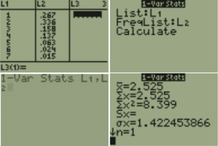
TI-84: Press [STAT], choose 1:Edit. For x and P(x) data pairs, enter all x-values in one list. Enter all corresponding P(x) values in a second list. Press [STAT]. Use cursor keys to highlight CALC. Select 1:1-Var Stats.

Enter list 1 for List and list 2 for frequency list. Press Enter to calculate the statistics. For TI-83, you will just see 1-Var Stats on the screen. Enter each list separated with a comma by pressing [2nd], then press the number 1 key corresponding to your x list, then a comma, then [2nd] and the number 2 key corresponding to your P(x) values. The home screen should look like this 1-Var Stats L₁,L₂.

TI-84 screens for a probability distribution: the list editor with values 1 through 7 in L1 and probabilities 0.267, 0.336, 0.158, 0.137, 0.063, 0.024, and 0.015 in L2; the 1-Var Stats setup with List L1 and FreqList L2; and results showing x̄ = 2.525, Σx = 2.525, Σx² = 8.399, σx = 1.422453866, and n = 1.

Where the calculator says $\bar{x}$ is µ the population mean and σ_x is the population standard deviation (square this number to get the population variance).

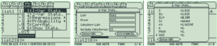
TI-89: Go to the [Apps] Stat/List Editor, and type the x values into List 1 and P(x) values into List2. Select F4 for the Calc menu. Use cursor keys to highlight 1:1-Var Stats.

Under List, press [2^nd] Var-Link, then select list1. Under Freq, press [2^nd] Var-Link, then select list2. Press enter twice and the statistics will appear in a new window.

Use the cursor keys to arrow up and down to see all of the values. Note: $\bar{x}$ this is µ the population mean and σx is the population standard deviation; square this value to get the variance.

TI-89 Stat/List Editor screens: the Calc menu listing 1-Var Stats, 2-Var Stats, Regressions, Probability, CorrMat, and Show Stats; the 1-Var Stats dialog with List set to list1 and Freq set to list2; and a results window showing x̄ = 2.525, Σx = 2.525, Σx² = 8.399, Sx undefined, σx = 1.42245, and n = 1.

Bernoulli trial

The focus of the previous section was on discrete probability distribution tables. To find the table for those situations, we usually need to actually conduct the experiment and collect data. Then one can calculate the experimental probabilities.

Jacob Bernoulli

If certain conditions are met, we can instead use theoretical probabilities. One of these theoretical probabilities can be used when we have a Bernoulli trial.

Properties of a Bernoulli trial or binomial trial:

Trials are independent, which means that what happens on one trial does not influence the outcomes of other trials.
There are only two outcomes, which are called a success and a failure.
The probability of a success does not change from trial to trial, where p = probability of success and q = probability of failure, the complement of p, q = 1 – p.

If you know you have a Bernoulli trial, then you can calculate probabilities using some theoretical probability formulas. This is important because Bernoulli trials come up often in real life.

Examples of Bernoulli experiments are:

Toss a fair coin twice, and find the probability of getting two heads.
Question twenty people in class, and look for the probability of more than half are business majors.
A patient has a virus.
What is the probability of passing a multiple-choice test if you have not studied?

Bernoulli trials are used in both the geometric and binomial distributions.

Adapted from Mostly Harmless Statistics by Rachel Webb (Portland State University), hosted on LibreTexts (stats.libretexts.org) and licensed under CC BY-SA 4.0. Changes were made. License: CC-BY-SA-4.0.