4.6 PDEs, Separation of Variables, and The Heat Equation

Let us recall that a partial differential equation or PDE is an equation containing the partial derivatives with respect to several independent variables. Solving PDEs will be our main application of Fourier series.

A PDE is said to be linear if the dependent variable and its derivatives appear at most to the first power and in no functions. We will only talk about linear PDEs. Together with a PDE, we usually have specified some boundary conditions, where the value of the solution or its derivatives is specified along the boundary of a region, and/or some initial conditions where the value of the solution or its derivatives is specified for some initial time. Sometimes such conditions are mixed together and we will refer to them simply as side conditions.

We will study three specific partial differential equations, each one representing a more general class of equations. First, we will study the heat equation, which is an example of a parabolic PDE. Next, we will study the wave equation, which is an example of a hyperbolic PDE. Finally, we will study the Laplace equation, which is an example of an elliptic PDE. Each of our examples will illustrate behavior that is typical for the whole class.

Heat on an Insulated Wire

Let us first study the heat equation. Suppose that we have a wire (or a thin metal rod) of length $L$ that is insulated except at the endpoints. Let $x$ denote the position along the wire and let $t$ denote time. See Figure $1$ .

Diagram of an insulated wire: a thin cylinder along the x-axis from 0 to L, capped at both ends, with a vertical axis at the left labelled temperature u. — Figure $1$ : Insulated wire.

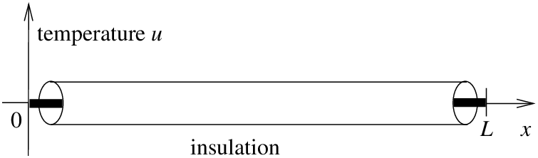
Let $u (x, t)$ denote the temperature at point $x$ at time $t$ . The equation governing this setup is the so-called one-dimensional heat equation:

$\frac{\partial u}{\partial t} = k \frac{\partial^{2} u}{\partial x^{2}},$

where $k greater than 0$ is a constant (the thermal conductivity of the material). That is, the change in heat at a specific point is proportional to the second derivative of the heat along the wire. This makes sense; if at a fixed $t$ the graph of the heat distribution has a maximum (the graph is concave down), then heat flows away from the maximum. And vice-versa.

We will generally use a more convenient notation for partial derivatives. We will write $u_{t}$ instead of $\frac{\partial u}{\partial t}$ , and we will write $u_{x x}$ instead of $\frac{\partial^{2} u}{\partial x^{2}}$ . With this notation the heat equation becomes

$u_{t} = k u_{x x} .$

For the heat equation, we must also have some boundary conditions. We assume that the ends of the wire are either exposed and touching some body of constant heat, or the ends are insulated. For example, if the ends of the wire are kept at temperature 0, then we must have the conditions

$u (0, t) = 0 and u (L, t) = 0 .$

If, on the other hand, the ends are also insulated we get the conditions

$u_{x} (0, t) = 0 and u_{x} (L, t) = 0 .$

Let us see why that is so. If $u_{x}$ is positive at some point $x sub 0$ , then at a particular time, $u$ is smaller to the left of $x sub 0$ , and higher to the right of $x sub 0$ . Heat is flowing from high heat to low heat, that is to the left. On the other hand if $u_{x}$ is negative then heat is again flowing from high heat to low heat, that is to the right. So when $u_{x}$ is zero, that is a point through which heat is not flowing. In other words, $u sub x open parenthesis 0, t close parenthesis equals 0$ means no heat is flowing in or out of the wire at the point $x equals 0$ .

We have two conditions along the $x$ -axis as there are two derivatives in the $x$ direction. These side conditions are said to be homogeneous (i.e., $u$ or a derivative of $u$ is set to zero).

We also need an initial condition—the temperature distribution at time $t equals 0$ . That is,

$u open parenthesis x, 0 close parenthesis equals f open parenthesis x close parenthesis,$

for some known function $f (x)$ . This initial condition is not a homogeneous side condition.

Separation of Variables

The heat equation is linear as $u$ and its derivatives do not appear to any powers or in any functions. Thus the principle of superposition still applies for the heat equation (without side conditions). If $u sub 1$ and $u sub 2$ are solutions and $c sub 1, c sub 2$ are constants, then $u = c_{1} u_{1} + c_{2} u_{2}$ is also a solution.

Superposition also preserves some of the side conditions. In particular, if $u sub 1$ and $u sub 2$ are solutions that satisfy $u open parenthesis 0, t close parenthesis equals 0$ and $u sub open parenthesis L, t close parenthesis equals 0$ , and $c sub 1, c sub 2$ are constants, then $u = c_{1} u_{1} + c_{2} u_{2}$ is still a solution that satisfies $u open parenthesis 0, t close parenthesis equals 0$ and $u sub open parenthesis L, t close parenthesis equals 0$ . Similarly for the side conditions $u sub x open parenthesis 0, t close parenthesis equals 0$ and $u sub x open parenthesis L, t close parenthesis equals 0$ . In general, superposition preserves all homogeneous side conditions.

The method of separation of variables is to try to find solutions that are sums or products of functions of one variable. For example, for the heat equation, we try to find solutions of the form

$u (x, t) = X (x) T (t) .$

That the desired solution we are looking for is of this form is too much to hope for. What is perfectly reasonable to ask, however, is to find enough “building-block” solutions of the form $u (x, t) = X (x) T (t)$ using this procedure so that the desired solution to the PDE is somehow constructed from these building blocks by the use of superposition.

Let us try to solve the heat equation

$u_{t} = k u_{x x} with u (0, t) = 0, u (L, t) = 0, and u (x, 0) = f (x) .$

Let us guess $u (x, t) = X (x) T (t)$ . We will try to make this guess satisfy the differential equation, $u_{t} = k u_{x x}$ , and the homogeneous side conditions, $u open parenthesis 0, t close parenthesis equals 0$ and $u open parenthesis L, t close parenthesis equals 0$ . Then, as superposition preserves the differential equation and the homogeneous side conditions, we will try to build up a solution from these building blocks to solve the nonhomogeneous initial condition $u open parenthesis x, 0 close parenthesis equals f open parenthesis x close parenthesis$ .

First we plug $u (x, t) = X (x) T (t)$ into the heat equation to obtain

$X (x) T^{'} (t) = k X^{″} (x) T (t) .$

We rewrite as

$\frac{T^{'} (t)}{k T (t)} = \frac{X^{″} (x)}{X (x)} .$

This equation must hold for all $x$ and all $t$ . But the left hand side does not depend on $x$ and the right hand side does not depend on $t$ . Hence, each side must be a constant. Let us call this constant $- λ$ (the minus sign is for convenience later). We obtain the two equations

$\frac{T^{'} (t)}{k T (t)} = - λ = \frac{X^{″} (x)}{X (x)} .$

In other words

$\begin{matrix} X^{″} (x) + λ X (x) = 0, \\ T^{'} (t) + λ k T (t) = 0 . \end{matrix}$

The boundary condition $u open parenthesis 0, t close parenthesis equals 0$ implies $X open parenthesis 0 close parenthesis T open parenthesis t close parenthesis equals 0$ . We are looking for a nontrivial solution and so we can assume that $T (t)$ is not identically zero. Hence $X open parenthesis 0 close parenthesis equals 0$ . Similarly, $u open parenthesis L, t close parenthesis equals 0$ implies $X open parenthesis L close parenthesis equals 0$ . We are looking for nontrivial solutions $X$ of the eigenvalue problem $X^{″} + λ X = 0, X (0) = 0, X (L) = 0$ . We have previously found that the only eigenvalues are $λ_{n} = \frac{n^{2} π^{2}}{L^{2}}$ , for integers $n greater than or equal to 1$ , where eigenfunctions are $\sin (\frac{n π}{L} x)$ . Hence, let us pick the solutions

$X_{n} (x) = \sin (\frac{n π}{L} x) .$

The corresponding $T_{n}$ must satisfy the equation

$T_{n}^{'} (t) + \frac{n^{2} π^{2}}{L^{2}} k T_{n} (t) = 0 .$

By the method of integrating factor, the solution of this problem is

$T_{n} (t) = e^{\frac{- n^{2} π^{2}}{L^{2}} k t} .$

It will be useful to note that $T sub n open parenthesis 0 close parenthesis equals 1$ . Our building-block solutions are

$u_{n} (x, t) = X_{n} (x) T_{n} (t) = \sin (\frac{n π}{L} x) e^{\frac{- n^{2} π^{2}}{L^{2}} k t} .$

We note that $u_{n} (x, 0) = \sin (\frac{n π}{L} x)$ . Let us write $f (x)$ as the sine series

$f (x) = \sum_{n = 1}^{\infty} b_{n} \sin (\frac{n π}{L} x) .$

That is, we find the Fourier series of the odd periodic extension of $f (x)$ . We used the sine series as it corresponds to the eigenvalue problem for $X (x)$ above. Finally, we use superposition to write the solution as

$u (x, t) = \sum_{n = 1}^{\infty} b_{n} u_{n} (x, t) = \sum_{n = 1}^{\infty} b_{n} \sin (\frac{n π}{L} x) e^{\frac{- n^{2} π^{2}}{L^{2}} k t} .$

Why does this solution work? First note that it is a solution to the heat equation by superposition. It satisfies $u open parenthesis 0, t close parenthesis equals 0$ and $u open parenthesis L, t close parenthesis equals 0$ , because $x equals 0$ or $x = L$ makes all the sines vanish. Finally, plugging in $t equals 0$ , we notice that $T sub n open parenthesis 0 close parenthesis equals 1$ and so

$u (x, 0) = \sum_{n = 1}^{\infty} b_{n} u_{n} (x, 0) = \sum_{n = 1}^{\infty} b_{n} \sin (\frac{n π}{L} x) = f (x) .$

Example 1

Suppose that we have an insulated wire of length $1$ , such that the ends of the wire are embedded in ice (temperature 0). Let $k equals 0.003$ . Then suppose that initial heat distribution is $u (x, 0) = 50 x (1 - x)$ . See Figure $2$ .

Figure

2

: Initial distribution of temperature in the wire.

We want to find the temperature function $u (x, t)$ . Let us suppose we also want to find when (at what $t$ ) does the maximum temperature in the wire drop to one half of the initial maximum of $12.5$ .

We are solving the following PDE problem:

$\begin{matrix} u_{t} = 0.003 u_{x x}, \\ u (0, t) = u (1, t) = 0, \\ u (x, 0) = 50 x (1 - x) f o r 0 < x < 1 . \end{matrix}$

We write $f (x) = 50 x (1 - x)$ for $0 less than x less than 1$ as a sine series. That is, $f (x) = \sum_{n = 1}^{\infty} b_{n} \sin (n π x)$ , where

$\begin{matrix} 0 i f n e v e n, \\ \frac{400}{π^{3} n^{3}} i f n o d d . \end{matrix}$

Figure

3

: Plot of the temperature of the wire at position

x

at time

t

The solution $u (x, t)$ , plotted in Figure $3$ for $ 0 \leq t \leq 100$, is given by the series:

$u (x, t) = \sum_{\underset{n o d d}{n = 1}}^{\infty} \frac{400}{π^{3} n^{3}} \sin (n π x) e^{- n^{2} π^{2} 0.003 t} .$

Finally, let us answer the question about the maximum temperature. It is relatively easy to see that the maximum temperature will always be at $x equals 0.5$ , in the middle of the wire. The plot of $u (x, t)$ confirms this intuition.

If we plug in $x equals 0.5$ we get

$u (0.5, t) = \sum_{\underset{n o d d}{n = 1}}^{\infty} \frac{400}{π^{3} n^{3}} \sin (n π 0.5) e^{- n^{2} π^{2} 0.003 t} .$

For $n equals 3$ and higher (remember $n$ is only odd), the terms of the series are insignificant compared to the first term. The first term in the series is already a very good approximation of the function. Hence

$u (0.5, t) \approx \frac{400}{π^{3}} e^{- π^{2} 0.003 t} .$

The approximation gets better and better as $t$ gets larger as the other terms decay much faster. Let us plot the function $0.5, t$ , the temperature at the midpoint of the wire at time $t$ , in Figure $4$ . The figure also plots the approximation by the first term.

Figure

4

: Temperature at the midpoint of the wire (the bottom curve), and the approximation of this temperature by using only the first term in the series (top curve).

After $t equals 5$ or so it would be hard to tell the difference between the first term of the series for $u (x, t)$ and the real solution $u (x, t)$ . This behavior is a general feature of solving the heat equation. If you are interested in behavior for large enough $t$ , only the first one or two terms may be necessary.

Let us get back to the question of when is the maximum temperature one half of the initial maximum temperature. That is, when is the temperature at the midpoint $12.5 / 2 equals 6.25$ . We notice on the graph that if we use the approximation by the first term we will be close enough. We solve

$6.25 = \frac{400}{π^{3}} e^{- π^{2} 0.003 t} .$

That is,

$t = \frac{\ln \frac{6.25 π^{3}}{400}}{- π^{2} 0.003} \approx 24.5 .$

So the maximum temperature drops to half at about $t equals 24.5$ .

We mention an interesting behavior of the solution to the heat equation. The heat equation “smoothes” out the function $f (x)$ as $t$ grows. For a fixed $t$ , the solution is a Fourier series with coefficients $b_{n} e^{\frac{- n^{2} π^{2}}{L^{2}} k t}$ . If $t greater than 0$ , then these coefficients go to zero faster than any $\frac{1}{n^{P}}$ for any power $p$ . In other words, the Fourier series has infinitely many derivatives everywhere. Thus even if the function $f (x)$ has jumps and corners, then for a fixed $t greater than 0$ , the solution $u (x, t)$ as a function of $x$ is as smooth as we want it to be.

Insulated Ends

Now suppose the ends of the wire are insulated. In this case, we are solving the equation

$u_{t} = k u_{x x} with u_{x} (0, t) = 0, u_{x} (L, t) = 0, and u (x, 0) = f (x) .$

Yet again we try a solution of the form $u (x, t) = X (x) T (t)$ . By the same procedure as before we plug into the heat equation and arrive at the following two equations

$\begin{matrix} X^{″} (x) + λ X (x) = 0, \\ T^{'} (t) + λ k T (t) = 0 . \end{matrix}$

At this point the story changes slightly. The boundary condition $u sub x open parenthesis 0, t close parenthesis equals 0$ implies $X prime open parenthesis 0 close parenthesis T open parenthesis t close parenthesis equals 0$ . Hence $X prime open parenthesis 0 close parenthesis equals 0$ . Similarly, $u sub x open parenthesis L, t close parenthesis equals 0$ implies $X prime open parenthesis L close parenthesis equals 0$ . We are looking for nontrivial solutions $X$ of the eigenvalue problem $X^{″} + λ X = 0,$ $X prime open parenthesis 0 close parenthesis equals 0,$ $X prime open parenthesis L close parenthesis equals 0,$ . We have previously found that the only eigenvalues are $λ_{n} = \frac{n^{2} π^{2}}{L^{2}}$ , for integers $n greater than or equal to 0$ , where eigenfunctions are $\cos (\frac{n π}{L}) X$ (we include the constant eigenfunction). Hence, let us pick solutions

$X_{n} (x) = \cos (\frac{n π}{L} x) and X_{0} (x) = 1 .$

The corresponding $T_{n}$ must satisfy the equation

$T_{n}^{'} (t) + \frac{n^{2} π^{2}}{L^{2}} k T_{n} (t) = 0 .$

For $n greater than or equal to 1$ , as before,

$T_{n} (t) = e^{\frac{- n^{2} π^{2}}{L^{2}} k t} .$

For $n equals 0$ , we have $T 0 ′ open parenthesis t close parenthesis equals 0$ and hence $T sub 0 open parenthesis t close parenthesis equals 1$ . Our building-block solutions will be

$u_{n} (x, t) = X_{n} (x) T_{n} (t) = \cos (\frac{n π}{L} x) e^{\frac{- n^{2} π^{2}}{L^{2}} k t},$

and

$u sub 0 open parenthesis x, t close parenthesis equals 1.$

We note that $u_{n} (x, 0) = \cos (\frac{n π}{L} x)$ . Let us write $f$ using the cosine series

$f (x) = \frac{a_{0}}{2} + \sum_{n = 1}^{\infty} a_{n} \cos (\frac{n π}{L} x) .$

That is, we find the Fourier series of the even periodic extension of $f (x)$ .

We use superposition to write the solution as

$u (x, t) = \frac{a_{0}}{2} + \sum_{n = 1}^{\infty} a_{n} u_{n} (x, t) = \frac{a_{0}}{2} + \sum_{n = 1}^{\infty} a_{n} \cos (\frac{n π}{L} x) e^{\frac{- n^{2} π^{2}}{L^{2}} k t} .$

Example 3

Let us try the same equation as before, but for insulated ends. We are solving the following PDE problem

$\begin{matrix} u_{t} = 0.003 u_{x x}, \\ u_{x} (0, t) = u_{x} (1, t) = 0, \\ u (x, 0) = 50 x (1 - x) f o r 0 < x < 1 . \end{matrix}$

For this problem, we must find the cosine series of $u open parenthesis x, 0 close parenthesis$ . For $0 less than x less than 1$ we have

$50 x (1 - x) = \frac{25}{3} + \sum_{\underset{n e v e n}{n = 2}}^{\infty} (\frac{- 200}{π^{2} n^{2}}) \cos (n π x) .$

The calculation is left to the reader. Hence, the solution to the PDE problem, plotted in Figure $5$ , is given by the series

$u (x, t) = \frac{25}{3} + \sum_{\underset{n e v e n}{n = 2}}^{\infty} (\frac{- 200}{π^{2} n^{2}}) \cos (n π x) e^{- n^{2} π^{2} 0.003 t} .$

Figure

5

: Plot of the temperature of the insulated wire at position

x

at time

t

Note in the graph that the temperature evens out across the wire. Eventually, all the terms except the constant die out, and you will be left with a uniform temperature of $\frac{25}{3} \approx{8.33}$ along the entire length of the wire.

Explore in 3D (opens in a new tab)

The temperature surface u(x, t) = e^(-0.3 n^2 t) sin(n x) for one term of the series, with time running along the second axis. Drag the mode-number slider: higher modes wiggle faster in x and die out much faster in t - the n^2 in the exponent is why only the low modes survive, and why the temperature evens out.

Let us expand on the last point. The constant term in the series is

$\frac{a_{0}}{2} = \frac{1}{L} \int_{0}^{L} f (x) d x .$

In other words,

\frac{a_{0}}{2}

is the average value of

f (x)

, that is, the average of the initial temperature. As the wire is insulated everywhere, no heat can get out, no heat can get in. So the temperature tries to distribute evenly over time, and the average temperature must always be the same, in particular it is always

\frac{a_{0}}{2}

. As time goes to infinity, the temperature goes to the constant

\frac{a_{0}}{2}

everywhere.

Adapted from Differential Equations for Engineers by Jiří Lebl (Oklahoma State University), hosted on LibreTexts (math.libretexts.org) and licensed under CC BY-SA 4.0. Changes were made. License: CC-BY-SA-4.0.