4.2 The Trigonometric Series

Periodic Functions and Motivation

As motivation for studying Fourier series, suppose we have the problem

$x^{″} + ω_{0}^{2} x = f (t),$

(4.2.1)

for some periodic function $f (t)$ . We have already solved

$x^{″} + ω_{0}^{2} x = F_{0} \cos (ω t) .$

(4.2.2)

One way to solve (4.2.1) is to decompose $f (t)$ as a sum of cosines (and sines) and then solve many problems of the form (4.2.2). We then use the principle of superposition, to sum up all the solutions we got to get a solution to (4.2.1).

Before we proceed, let us talk a little bit more in detail about periodic functions. A function is said to be periodic with period $P$ if $f (t)$ for all $t$ . For brevity we will say $f (t)$ is $P -$ periodic. Note that a $P -$ periodic function is also $2 P minus$ periodic, $3 P minus$ periodic and so on. For example, $\cos (t)$ and $\sin (t)$ are $2 π minus$ periodic. So are $\cos (k t)$ and $\sin (k t)$ for all integers $k$ . The constant functions are an extreme example. They are periodic for any period (exercise).

Normally we will start with a function $f (t)$ defined on some interval $[ minus L, L ]$ and we will want to extend $f (t)$ periodically to make it a $2 L minus$ periodic function. We do this extension by defining a new function $F (t)$ such that for $t$ in $[ minus L, L ]$ , $F (t) = f (t)$ . For $t$ in $[ L, 3 L ]$ , we define $F (t) = f (t - 2 L)$ , for $t$ in $[- 3 L, - L]$ , $F (t) = f (t + 2 L)$ , and so on. We assumed that $f (- L) = f (L)$ . We could have also started with $f$ defined only on the half-open interval $open parenthesis minus L, L ]$ and then define $f (- L) = f (L)$ .

You should be careful to distinguish between $f (t)$ and its extension. A common mistake is to assume that a formula for $f (t)$ holds for its extension. It can be confusing when the formula for $f (t)$ is periodic, but with perhaps a different period.

Inner Product and Eigenvector Decomposition

Suppose we have a symmetric matrix, that is $A^{T} = A$ . We have said before that the eigenvectors of $A$ are then orthogonal. Here the word orthogonal means that if $\vec{v}$ and $\vec{w}$ are two distinct (and not multiples of each other) eigenvectors of $A$ , then $⟨ v →, w → ⟩ equals 0$ . In this case the inner product $⟨ \vec{v}, \vec{w} ⟩$ is the dot product, which can be computed as ${\vec{v}}^{T} \vec{w}$ .

To decompose a vector $\vec{v}$ in terms of mutually orthogonal vectors $w → sub 1$ and $w → sub 2$ we write

$\vec{v} = a_{1} {\vec{w}}_{1} + a_{2} {\vec{w}}_{2} .$

Let us find the formula for $a sub 1$ and $a sub 2$ . First let us compute

$⟨ \vec{v}, \vec{w_{1}} ⟩ = ⟨ a_{1} {\vec{w}}_{1} + a_{2} {\vec{w}}_{2}, \vec{w_{1}} ⟩ = a_{1} ⟨ {\vec{w}}_{1}, \vec{w_{1}} ⟩ + a_{2} \underset{= 0}{\underset{⏟}{⟨ {\vec{w}}_{2}, \vec{w_{1}} ⟩}} = a_{1} ⟨ {\vec{w}}_{1}, \vec{w_{1}} ⟩ .$

Therefore,

$a_{1} = \frac{⟨ \vec{v}, {\vec{w}}_{1} ⟩}{⟨ {\vec{w}}_{1}, {\vec{w}}_{1} ⟩} .$

Similarly

$a_{2} = \frac{⟨ \vec{v}, {\vec{w}}_{2} ⟩}{⟨ {\vec{w}}_{2}, {\vec{w}}_{2} ⟩} .$

You probably remember this formula from vector calculus.

Example 2

Write $2; 3$ as a linear combination of $1; minus 1$ and $1; 1$ .

First note that $w → sub 1$ and $w → sub 2$ are orthogonal as $⟨ {\vec{w}}_{1}, {\vec{w}}_{2} ⟩ = 1 (1) + (- 1) 1 = 0$ . Then

$\begin{matrix} a_{1} = \frac{⟨ \vec{v}, {\vec{w}}_{1} ⟩}{⟨ {\vec{w}}_{1}, {\vec{w}}_{1} ⟩} = \frac{2 (1) + 3 (- 1)}{1 (1) + (- 1) (- 1)} = \frac{- 1}{2}, \\ a_{2} = \frac{⟨ \vec{v}, {\vec{w}}_{2} ⟩}{⟨ {\vec{w}}_{2}, {\vec{w}}_{2} ⟩} = \frac{2 + 3}{1 + 1} = \frac{5}{2} . \end{matrix}$

Hence

$2; 3$

Trigonometric Series

Instead of decomposing a vector in terms of eigenvectors of a matrix, we will decompose a function in terms of eigenfunctions of a certain eigenvalue problem. The eigenvalue problem we will use for the Fourier series is

$x^{″} + λ x = 0, x (- π) = x (π) x^{'} (- π) = x^{'} (π) .$

We have previously computed that the eigenfunctions are $1, cos open parenthesis k t close parenthesis, sin open parenthesis k t close parenthesis$ . That is, we will want to find a representation of a $2 π minus$ periodic function $f (t)$ as

$f (t) = \frac{a_{0}}{2} + \sum_{n = 1}^{\infty} a_{n} \cos (n t) + b_{n} \sin (n t) .$

This series is called the Fourier seriesto the power 1 or the trigonometric series for $f (t)$ . We write the coefficient of the eigenfunction $1$ as $\frac{a_{0}}{2}$ for convenience. We could also think of $1 equals cos open parenthesis 0 t close parenthesis$ , so that we only need to look at $\cos (k t)$ and $\sin (k t)$ .

As for matrices we want to find a projection of $f (t)$ onto the subspace generated by the eigenfunctions. So we will want to define an inner product of functions. For example, to find $a_{n}$ we want to compute $⟨ f (t), \cos (n t) ⟩$ . We define the inner product as

$⟨ f (t), g (t) ⟩ = \int_{- π}^{π} f (t) g (t) d t .$

With this definition of the inner product, we have seen in the previous section that the eigenfunctions $\cos (k t)$ (including the constant eigenfunction), and $\sin (k t)$ are orthogonal in the sense that

$\begin{matrix} ⟨ \cos (m t), \cos (n t) ⟩ = 0 for m ⧸ = n, \\ ⟨ \sin (m t), \sin (n t) ⟩ = 0 for m ⧸ = n, \\ ⟨ \sin (m t), \cos (n t) ⟩ = 0 for all m and n . \end{matrix}$

By elementary calculus for $n equals 1, 2, 3, ….$ we have $⟨ \cos (n t), \cos (n t) ⟩ = π$ and $⟨ \sin (n t), \sin (n t) ⟩ = π$ . For the constant we get

$⟨ 1, 1 ⟩ = \int_{π}^{π} 1 \cdot 1 d t = 2 π .$

The coefficients are given by

$\begin{matrix} a_{n} = \frac{⟨ f (t), \cos (n t) ⟩}{⟨ \cos (n t), \cos (n t) ⟩} = \frac{1}{π} \int_{- π}^{π} f (t) \cos (n t) d t, \\ b_{n} = \frac{⟨ f (t), \sin (n t) ⟩}{⟨ \sin (n t), \sin (n t) ⟩} = \frac{1}{π} \int_{- π}^{π} f (t) \sin (n t) d t . \end{matrix}$

Compare these expressions with the finite-dimensional example. For $a sub 0$ we get a similar formula

$a_{0} = 2 \frac{⟨ f (t), 1 ⟩}{⟨ 1, 1 ⟩} \frac{1}{π} \int_{- π}^{π} f (t) d t .$

Let us check the formulas using the orthogonality properties. Suppose for a moment that

$f (t) = \frac{a_{0}}{2} + \sum_{n = 1}^{\infty} a_{n} \cos (n t) + b_{n} \sin (n t) .$

Then for $m greater than or equal to 1$ we have

$\begin{matrix} ⟨ f (t), \cos (m t) ⟩ = ⟨ \frac{a_{0}}{2} + \sum_{n = 1}^{\infty} a_{n} \cos (n t) + b_{n} \sin (n t), \cos (m t) ⟩ \\ = \frac{a_{0}}{2} ⟨ 1, \cos (m t) ⟩ + \sum_{n = 1}^{\infty} a_{n} ⟨ \cos (n t), \cos (m t) ⟩ + b_{n} ⟨ \sin (n t), \sin (m t) ⟩ \\ = a_{m} ⟨ \cos (m t), \cos (m t) ⟩ . \end{matrix}$

And hence $a_{m} = \frac{⟨ f (t), \cos (m t) ⟩}{⟨ \cos (m t), \cos (m t) ⟩} .$

Example 3

Take the function

$f (t) = t$

for $t$ in $open parenthesis minus π, π ]$ . Extend $f (t)$ periodically and write it as a Fourier series. This function is called the sawtooth.

The plot of the extended periodic function is given in Figure $2$ . Let us compute the coefficients.

Figure

2

: The graph of the sawtooth function.

Show solution

We start with $a sub 0$ ,

$a_{0} = \frac{1}{π} \int_{- π}^{π} t d t = 0 .$

We will often use the result from calculus that says that the integral of an odd function over a symmetric interval is zero. Recall that an odd function is a function $φ (t)$ such that $φ (- t) = - φ (t)$ . For example the functions $t, \sin t$ , or (importantly for us) $t \cos (n t)$ are all odd functions. Thus

$a_{n} = \frac{1}{π} \int_{- π}^{π} t \cos (n t) d t = 0 .$

Let us move to $b_{n}$ . Another useful fact from calculus is that the integral of an even function over a symmetric interval is twice the integral of the same function over half the interval. Recall an even function is a function $φ (t)$ such that $φ (- t) = φ (t)$ . For example $t \sin (n t)$ is even.

$\begin{matrix} b_{n} = \frac{1}{π} \int_{- π}^{π} t \sin (n t) d t \\ = \frac{2}{π} \int_{0}^{π} t \sin (n t) d t \\ = \frac{2}{π} ({[\frac{- t \cos (n t)}{n}]}_{t = 0}^{π} + \frac{1}{n} \int_{0}^{π} \cos (n t) d t) \\ = \frac{2}{π} (\frac{- π \cos (n π)}{n} + 0) \\ = \frac{- 2 \cos (n π)}{n} = \frac{2 (- 1)^{n + 1}}{n} . \end{matrix}$

We have used the fact that

$1 i f n e v e n,; minus 1 i f n o d d.$

The series, therefore, is

$\sum_{n = 1}^{\infty} \frac{2 (- 1)^{n + 1}}{n} \sin (n t) .$

Let us write out the first $3$ harmonics of the series for $f (t)$ .

$2 \sin (t) - \sin (2 t) + \frac{2}{3} \sin (3 t) + \dots$

The plot of these first three terms of the series, along with a plot of the first $20$ terms is given in Figure $3$ .

Figure

3

: First 3 (left graph) and 20 (right graph) harmonics of the sawtooth function.

Example 4

Take the function

$0 i f minus π less than t less than or equal to 0,; π i f 0 less than t less than or equal to π.$

Extend $f (t)$ periodically and write it as a Fourier series. This function or its variants appear often in applications and the function is called the square wave.

Figure

4

: The graph of the square wave function.

The plot of the extended periodic function is given in Figure $4$ . Now we compute the coefficients. Let us start with $a sub 0$

$a_{0} = \frac{1}{π} \int_{- π}^{π} f (t) d t = \frac{1}{π} \int_{0}^{π} π d t = π .$

Next,

$a_{n} = \frac{1}{π} \int_{- π}^{π} f (t) \cos (n t) d t = \frac{1}{π} \int_{0}^{π} π \cos (n t) d t = 0 .$

And finally

$\begin{matrix} b_{n} = \frac{1}{π} \int_{- π}^{π} f (t) \sin (n t) d t \\ = \frac{1}{π} \int_{0}^{π} π \sin (n t) d t \\ = {[\frac{- \cos (n t)}{n}]}_{t = 0}^{π} \\ = \frac{1 - \cos (π n)}{n} = \frac{1 - (- 1)^{n}}{n} = {\begin{matrix} \frac{2}{n} i f n i s o d d, \\ 0 i f n i s e v e n . \end{matrix} \end{matrix}$

The Fourier series is

$\frac{π}{2} + \sum_{n = 1 n o d d}^{\infty} \frac{2}{n} \sin (n t) + \sum_{k = 1}^{\infty} \frac{2}{2 k - 1} \sin ((2 k - 1) t) .$

Let us write out the first 3 harmonics of the series for $f (t)$ .

$\frac{π}{2} + 2 \sin (t) + \frac{2}{3} \sin (3 t) + \dots$

The plot of these first three and also of the first 20 terms of the series is given in Figure $5$ .

Figure

5

: First 3 (left graph) and 20 (right graph) harmonics of the square wave function.

We have so far skirted the issue of convergence. For example, if $f (t)$ is the square wave function, the equation

$f (t) = \frac{π}{2} + \sum_{k = 1}^{\infty} \frac{2}{2 k - 1} \sin ((2 k - 1) t) .$

is only an equality for such $t$ where $f (t)$ is continuous. That is, we do not get an equality for $t = - π, 0, π$ and all the other discontinuities of $f (t)$ . It is not hard to see that when $t$ is an integer multiple of $π$ (which includes all the discontinuities), then

$\frac{π}{2} + \sum_{k = 1}^{\infty} \frac{2}{2 k - 1} \sin ((2 k - 1) t) = \frac{π}{2} .$

We redefine $f (t)$ on $[ minus π, π ]$ as

$\begin{matrix} 0 i f - π < t < 0, \\ π i f 0 < t < π, \\ π / 2 i f t = - π, t = 0, o r t = π, \end{matrix}$

and extend periodically. The series equals this extended $f (t)$ everywhere, including the discontinuities. We will generally not worry about changing the function values at several (finitely many) points.

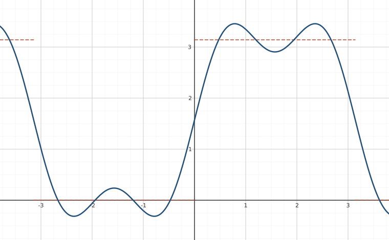
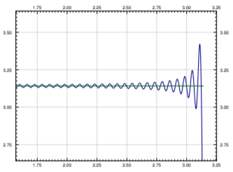
We will say more about convergence in the next section. Let us however mention briefly an effect of the discontinuity. Let us zoom in near the discontinuity in the square wave. Further, let us plot the first 100 harmonics, see Figure $6$ . You will notice that while the series is a very good approximation away from the discontinuities, the error (the overshoot) near the discontinuity at $t = π$ does not seem to be getting any smaller. This behavior is known as the Gibbs phenomenon. The region where the error is large does get smaller, however, the more terms in the series we take.

Function graph showing y = (pi/2)*(1+sign(sin(t))) and y = pi/2 + (1+sign(n-0.5))/1*sin(1*t) + (1+sign(n-2.5))/3*sin(3*t) + (1+sign(n-4.5))/5*sin(5*t) + (1+sign(n-6.5))/7*sin(7*t) + (1+sign(n-8.5))/9*sin(9*t) + (1+sign(n-10.5))/11*sin(11*t) + (1+sign(n-12.5))/13*sin(13*t) + (1+sign(n-14.5))/15*sin(15*t) + (1+sign(n-16.5))/17*sin(17*t) + (1+sign(n-18.5))/19*sin(19*t) + (1+sign(n-20.5))/21*sin(21*t) + (1+sign(n-22.5))/23*sin(23*t) + (1+sign(n-24.5))/25*sin(25*t) + (1+sign(n-26.5))/27*sin(27*t) + (1+sign(n-28.5))/29*sin(29*t) + (1+sign(n-30.5))/31*sin(31*t) + (1+sign(n-32.5))/33*sin(33*t) + (1+sign(n-34.5))/35*sin(35*t) + (1+sign(n-36.5))/37*sin(37*t) + (1+sign(n-38.5))/39*sin(39*t). Adjustable parameter: Highest harmonic kept (n) = 3. Viewing window: x from -3.8 to 3.8, y from -0.78 to 3.92. — Lebl's Figure 5 freezes this at two settings, 3 harmonics and 20; here you can sweep between them and past them. The dashed trace is the square wave itself; the solid curve is the partial sum of his own series pi/2 + 2 sin t + (2/3) sin 3t + (2/5) sin 5t +.... At the default 3 you are looking at his left-hand panel exactly, and at 20 at his right-hand one. Drag between them and the ripples multiply and crowd in toward the jumps at t = 0 and t = +/- pi, but the tall spike beside each jump refuses to come down: its peak falls only from 3.456 to 3.424 across that whole drag, and never drops below 3.4227 = 1.0895*pi -- a permanent overshoot of 8.95 % of the jump height pi. Even-numbered settings look identical to the odd one below them, because a square wave has no even harmonics at all: this section computes b_n = 0 for every even n.

Close-up of the Gibbs phenomenon: the blue partial sum ripples about a flat green line at the true value of about 3.14, the wiggles growing toward the jump until the tallest reaches roughly 3.42. — Figure $6$ : Gibbs phenomenon in action.

We can think of a periodic function as a “signal” being a superposition of many signals of pure frequency. For example, we could think of the square wave as a tone of certain base frequency. This base frequency is called the fundamental frequency. The square wave will be a superposition of many different pure tones of frequencies that are multiples of the fundamental frequency. In music, the higher frequencies are called the overtones. All the frequencies that appear are called the spectrum of the signal. On the other hand a simple sine wave is only the pure tone (no overtones). The simplest way to make sound using a computer is the square wave, and the sound is very different from a pure tone. If you ever played video games from the 1980s or so, then you heard what square waves sound like.

Footnotes

[1] Named after the French mathematician Jean Baptiste Joseph Fourier (1768 – 1830).

Adapted from Differential Equations for Engineers by Jiří Lebl (Oklahoma State University), hosted on LibreTexts (math.libretexts.org) and licensed under CC BY-SA 4.0. Changes were made. License: CC-BY-SA-4.0.