Before we tackle the Fourier series, we need to study the so-called boundary value problems (or endpoint problems). For example, suppose we have
for some constant , where is defined for in the interval . Unlike before, when we specified the value of the solution and its derivative at a single point, we now specify the value of the solution at two different points. Note that is a solution to this equation, so existence of solutions is not an issue here. Uniqueness of solutions is another issue. The general solution to has two arbitrary constants present.1 It is, therefore, natural (but wrong) to believe that requiring two conditions guarantees a unique solution.
What is going on? We will be interested in finding which constants allow a nonzero solution, and we will be interested in finding those solutions. This problem is an analogue of finding eigenvalues and eigenvectors of matrices.
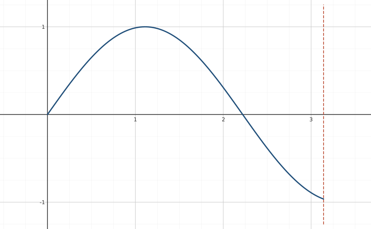
Interactive figureBoundary value problem x″ + λx = 0: which λ are eigenvalues?Drag the λ in x″ + λx = 0 slider from 0 to 17.
XYZ Graph · viewer build 5edf91b
Every λ makes x = sin(√λ t) satisfy the left condition x(0) = 0, so only the right endpoint is ever in play. Drag λ from 0 to 17 and watch where the curve meets the dashed line t = π: it lands on the axis exactly four times, at λ = 1, 4, 9 and 16 — the eigenvalues k² — and misses at every value in between, including Lebl's λ = 2 shown here. Below λ = 1 the curve never gets back down to the axis at all, and at λ = 0 it lies flat along the axis — no nonzero solution survives, which is why Lebl rules 0 out as an eigenvalue as well.
Eigenvalue Problems
For basic Fourier series theory we will need the following three eigenvalue problems. We will consider more general equations, but we will postpone this until Chapter 5.
(4.1.1)
and
(4.1.3)
A number is called an eigenvalue of (4.1.1) (resp. (4.1.2) or (4.1.3)) if and only if there exists a nonzero (not identically zero) solution to (4.1.1) (resp. (4.1.2) or (4.1.3)) given that specific . The nonzero solution we found is called the corresponding eigenfunction.
Note the similarity to eigenvalues and eigenvectors of matrices. The similarity is not just coincidental. If we think of the equations as differential operators, then we are doing the same exact thing. Think of a function as a vector with infinitely many components (one for each ). Let be the linear operator. Then the eigenvalue/eigenfunction pair should be and nonzero such that . In other words, we are looking for nonzero functions satisfying certain endpoint conditions that solve . A lot of the formalism from linear algebra still applies here, though we will not pursue this line of reasoning too far.
The following problem is the one that leads to the general Fourier series.
Orthogonality of Eigenfunctions
Something that will be very useful in the next section is the orthogonality property of the eigenfunctions. This is an analogue of the following fact about eigenvectors of a matrix. A matrix is called symmetric if . Eigenvectors for two distinct eigenvalues of a symmetric matrix are orthogonal. That symmetry is required. We will not prove this fact here. The differential operators we are dealing with act much like a symmetric matrix. We, therefore, get the following theorem.
Note that the terminology comes from the fact that the integral is a type of inner product. We will expand on this in the next section. The theorem has a very short, elegant, and illuminating proof so let us give it here. First note that we have the following two equations.
Multiply the first by and the second by and subtract to get
Now integrate both sides of the equation.
The last equality holds because of the boundary conditions. For example, if we consider (4.1.1) we have and so is zero at both and . As , the theorem follows.
We have seen previously that was an eigenfunction for the problem . Hence we have the integral
Similarly,
And finally we also get
and
Fredholm Alternative
We now touch on a very useful theorem in the theory of differential equations. The theorem holds in a more general setting than we are going to state it, but for our purposes the following statement is sufficient. We will give a slightly more general version in Chapter 5.
The theorem is also true for the other types of boundary conditions we considered. The theorem means that if is not an eigenvalue, the nonhomogeneous equation (4.1.4) has a unique solution for every right hand side. On the other hand if is an eigenvalue, then (4.1.4) need not have a solution for every , and furthermore, even if it happens to have a solution, the solution is not unique.
We also want to reinforce the idea here that linear differential operators have much in common with matrices. So it is no surprise that there is a finite dimensional version of Fredholm alternative for matrices as well. Let be an matrix. The Fredholm alternative then states that either has a nontrivial solution, or has a solution for every .
A lot of intuition from linear algebra can be applied to linear differential operators, but one must be careful of course. For example, one difference we have already seen is that in general a differential operator will have infinitely many eigenvalues, while a matrix has only finitely many.
Application
Let us consider a physical application of an endpoint problem. Suppose we have a tightly stretched quickly spinning elastic string or rope of uniform linear density . Let us put this problem into the plane. The axis represents the position on the string. The string rotates at angular velocity , so we will assume that the whole plane rotates at angular velocity . We will assume that the string stays in this plane and will measure its deflection from the equilibrium position, , on the axis. Hence, we will find a graph giving the shape of the string. We will idealize the string to have no volume to just be a mathematical curve. If we take a small segment and we look at the tension at the endpoints, we see that this force is tangential and we will assume that the magnitude is the same at both end points. Hence the magnitude is constant everywhere and we will call its magnitude . If we assume that the deflection is small, then we can use Newton’s second law to get an equation
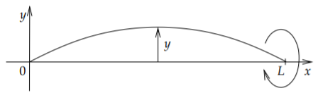
Let be the length of the string and the string is fixed at the beginning and end points. Hence, and . See Figure .
Figure : Whirling string.
We rewrite the equation as . The setup is similar to Example , except for the interval length being instead of . We are looking for eigenvalues of where . As before there are no nonpositive eigenvalues. With , the general solution to the equation is . The condition implies that as before. The condition implies that and hence for some integer , so
What does this say about the shape of the string? It says that for all parameters , , not satisfying the equation above, the string is in the equilibrium position, . When , then the string will some distance . We cannot compute with the information we have.
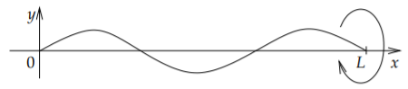
Let us assume that and are fixed and we are changing . For most values of the string is in the equilibrium state. When the angular velocity hits a value , then the string pops out and has the shape of a sin wave crossing the -axis times between the end points. For example, at , the string does not cross the -axis and the shape looks like in Figure . On the other hand, when the string crosses the -axis 2 times, see Figure . When changes again, the string returns to the equilibrium position. The higher the angular velocity, the more times it crosses the -axis when it is popped out.
Figure : Whirling string at the third eigenvalue .
For another example, if you have a spinning jump rope (then as it is completely ) and you pull on the ends to increase the tension, then the velocity also increases for the rope to stay "popped out".
Footnotes
[1] See Example 2.2.1 and Example 2.2.3.
[2] Recall that and . As an exercise try the computation with the general solution written as (for different and of course).
[3] Named after the Swedish mathematician Erik Ivar Fredholm (1866–1927).
These eBooks are a prerelease and are not yet certified conformant with WCAG 2.1 AA or ADA Title II. Every page is built against an automated accessibility gate, and the published editions will meet ADA Title II requirements when they release in late September 2026. If something is unusable, please tell us.