4.5 Applications of Fourier Series

Periodically Forced Oscillation

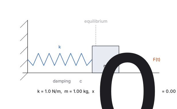
Let us return to the forced oscillations. Consider a mass-spring system as before, where we have a mass $m$ on a spring with spring constant $k$ , with damping $c$ , and a force $F (t)$ applied to the mass. Suppose the forcing function $F (t)$ is $2 L$ -periodic for some $L greater than 0$ . We have already seen this problem in chapter 2 with a simple $F (t)$ .

Diagram of a block m joined to a fixed wall by a spring k, with a bold arrow labelled F of t pushing right on the block and damping c marked along the surface beneath. — Figure $1$

The equation that governs this particular setup is

$m x^{″} (t) + c x^{'} (t) + k x (t) = F (t) .$

(4.5.1)

The general solution consists of (4.5.1) consists of the complementary solution $x_{c}$ , which solves the associated homogeneous equation $m x^{″} + c x^{'} + k x = 0$ , and a particular solution of Equation (4.5.1) we call $x_{p}$ . For $c greater than 0$ , the complementary solution $x_{c}$ will decay as time goes by. Therefore, we are mostly interested in a particular solution $x_{p}$ that does not decay and is periodic with the same period as $F (t)$ . We call this particular solution the steady periodic solution and we write it as $x_{s p}$ as before. What will be new in this section is that we consider an arbitrary forcing function $F (t)$ instead of a simple cosine.

For simplicity, let us suppose that $c equals 0$ . The problem with $c greater than 0$ is very similar. The equation

$m x^{″} + k x = 0$

has the general solution

$x (t) = A \cos (ω_{0} t) + B \sin (ω_{0} t),$

where $ω_{0} = \sqrt{\frac{k}{m}}$ . Any solution to $m x^{″} (t) + k x (t) = F (t)$ is of the form $A \cos (ω_{0} t) + B \sin (ω_{0} t) + x_{s p}$ . The steady periodic solution $x_{s p}$ has the same period as $F (t)$ .

In the spirit of the last section and the idea of undetermined coefficients we first write

$F (t) = \frac{c_{0}}{2} + \sum_{n = 1}^{\infty} c_{n} \cos (\frac{n π}{L} t) + d_{n} \sin (\frac{n π}{L} t) .$

Then we write a proposed steady periodic solution $x$ as

$x (t) = \frac{a_{0}}{2} + \sum_{n = 1}^{\infty} a_{n} \cos (\frac{n π}{L} t) + b_{n} \sin (\frac{n π}{L} t),$

where $a_{n}$ and $b_{n}$ are unknowns. We plug $x$ into the differential equation and solve for $a_{n}$ and $b_{n}$ in terms of $c_{n}$ and $d_{n}$ . This process is perhaps best understood by example.

Example 1

Suppose that $k equals 2$ , and $m equals 1$ . The units are again the mks units (meters-kilograms-seconds). There is a jetpack strapped to the mass, which fires with a force of 1 newton for 1 second and then is off for 1 second, and so on. We want to find the steady periodic solution.

Show solution

The equation is, therefore,

$x^{″} + 2 x = F (t),$

where $F (t)$ is the step function

$0 i f minus 1 less than t less than 0,; 1 i f 0 less than t less than 1,$

extended periodically. We write

$F (t) = \frac{c_{0}}{2} + \sum_{n = 1}^{\infty} c_{n} \cos (n π t) + d_{n} \sin (n π t) .$

We compute

$\begin{matrix} c_{n} = \int_{- 1}^{1} F (t) \cos (n π t) d t = \int_{0}^{1} \cos (n π t) d t = 0 f o r n \geq 1, \\ c_{0} = \int_{- 1}^{1} F (t) d t = \int_{0}^{1} d t = 1, \\ d_{n} = \int_{- 1}^{1} F (t) \sin (n π t) d t \\ = \int_{0}^{1} \sin (n π t) d t \\ = {[\frac{- \cos (n π t)}{n π}]}_{t = 0}^{1} \\ = \frac{1 - (- 1)^{n}}{π n} = {\begin{matrix} \frac{2}{π n} & i f n o d d, \\ 0 & i f n e v e n . \end{matrix} \end{matrix}$

$F (t) = \frac{1}{2} + \sum_{\underset{n o d d}{n = 1}}^{\infty} \frac{2}{π n} \sin (n π t) .$

We want to try

$x (t) = \frac{a_{0}}{2} + \sum_{n = 1}^{\infty} a_{n} \cos (n π t) + b_{n} \sin (n π t) .$

Once we plug into the differential equation $x^{″} + 2 x = F (t)$ , it is clear that $a sub n equals 0$ for $n greater than or equal to 1$ as there are no corresponding terms in the series for $F (t)$ . Similarly $b sub n equals 0$ for $n$ even. Hence we try

$x (t) = \frac{a_{0}}{2} + \sum_{\underset{n o d d}{n = 1}}^{\infty} b_{n} \sin (n π t) .$

We plug into the differential equation and obtain

$\begin{matrix} x^{″} + 2 x = \sum_{\underset{n o d d}{n = 1}}^{\infty} [- b_{n} n^{2} π^{2} \sin (n π t)] + a_{0} + 2 \sum_{\underset{n o d d}{n = 1}}^{\infty} [b_{n} \sin (n π t)] \\ = a_{0} + \sum_{\underset{n o d d}{n = 1}}^{\infty} b_{n} (2 - n^{2} π^{2}) \sin (n π t) \\ = F (t) = \frac{1}{2} + \sum_{\underset{n o d d}{n = 1}}^{\infty} \frac{2}{π n} \sin (n π t) . \end{matrix}$

So $a_{0} = \frac{1}{2}$ , $b sub n equals 0$ for even $n$ , and for odd $n$ we get

$b_{n} = \frac{2}{π n (2 - n^{2} π^{2})} .$

The steady periodic solution has the Fourier series

$x_{s p} (t) = \frac{1}{4} + \sum_{\underset{n o d d}{n = 1}}^{\infty} \frac{2}{π n (2 - n^{2} π^{2})} \sin (n π t) .$

We know this is the steady periodic solution as it contains no terms of the complementary solution and it is periodic with the same period as $F (t)$ itself. See Figure $1$ for the plot of this solution.

Figure

1

: Plot of the steady periodic solution

x_{s p}

of Example

1

Resonance

Just like when the forcing function was a simple cosine, resonance could still happen. Let us assume $c equals 0$ and we will discuss only pure resonance. Again, take the equation

$m x^{″} (t) + k x (t) = F (t) .$

When we expand $F (t)$ and find that some of its terms coincide with the complementary solution to $m x^{″} + k x = 0$ , we cannot use those terms in the guess. Just like before, they will disappear when we plug into the left hand side and we will get a contradictory equation (such as $0 equals 1$ ). That is, suppose

$x_{c} = A \cos (ω_{0} t) + B \sin (ω_{0} t),$

where $ω_{0} = \frac{N π}{L}$ for some positive integer $N$ . In this case we have to modify our guess and try

$x (t) = \frac{a_{0}}{2} + t (a_{N} \cos (\frac{N π}{L} t) + b_{N} \sin (\frac{N π}{L} t)) + \sum_{\underset{n \neq N}{n = 1}}^{\infty} a_{n} \cos (\frac{n π}{L} t) + b_{n} \sin (\frac{n π}{L} t) .$

In other words, we multiply the offending term by $t$ . From then on, we proceed as before.

Of course, the solution will not be a Fourier series (it will not even be periodic) since it contains these terms multiplied by $t$ . Further, the terms $t (a_{N} \cos (\frac{N π}{L} t) + b_{N} \sin (\frac{N π}{L} t))$ will eventually dominate and lead to wild oscillations. As before, this behavior is called pure resonance or just resonance.

Note that there now may be infinitely many resonance frequencies to hit. That is, as we change the frequency of $F$ (we change $L$ ), different terms from the Fourier series of $F$ may interfere with the complementary solution and will cause resonance. However, we should note that since everything is an approximation and in particular $c$ is never actually zero but something very close to zero, only the first few resonance frequencies will matter.

Example 2

Find the steady periodic solution to the equation

$2 x^{″} + 18 π^{2} x = F (t),$

(4.5.2)

where

$\begin{matrix} - 1 i f - 1 < t < 0, \\ 1 i f 0 < t < 1, \end{matrix}$

extended periodically. We note that

$F (t) = \sum_{\underset{n o d d}{n = 1}}^{\infty} \frac{4}{π n} \sin (n π t) .$

As $\sqrt{\frac{k}{m}} = \sqrt{\frac{18 π^{2}}{2}} = 3 π$ , the solution to (4.5.2) is

$x (t) = c_{1} \cos (3 π t) + c_{2} \sin (3 π t) + x_{p} (t)$

for some particular solution $x_{p}$ .

If we just try an $x_{p}$ given as a Fourier series with $\sin (n π t)$ as usual, the complementary equation, $2 x^{″} + 18 π^{2} x = 0$ , eats our $3 to the power rd$ harmonic. That is, the term with $sin open parenthesis 3 π t close parenthesis$ is already in in our complementary solution. Therefore, we pull that term out and multiply it by $t$ . We also add a cosine term to get everything right. That is, we try

$x_{p} (t) = a_{3} t \cos (3 π t) + b_{3} t \sin (3 π t) + \sum_{\underset{\underset{n \neq 3}{n o d d}}{n = 1}}^{\infty} b_{n} \sin (n π t) .$

Let us compute the second derivative.

${x_{p}^{'}}^{'} (t) = - 6 a_{3} π \sin (3 π t) - 9 π^{2} a_{3} t \cos (3 π t) + 6 b_{3} π \cos (3 π t) - 9 π^{2} b_{3} t \sin (3 π t) + \sum_{\underset{\underset{n \neq 3}{n o d d}}{n = 1}}^{\infty} (- n^{2} π^{2} b_{n}) \sin (n π t) .$

We now plug into the left hand side of the differential equation.

$\begin{matrix} 2 {x_{p}^{'}}^{'} + 18 π^{2} x_{p} = - 12 a_{3} π \sin (3 π t) - 18 π^{2} a_{3} t \cos (3 π t) + 12 b_{3} π \cos (3 π t) - 18 π^{2} b_{3} t \sin (3 π t) \\ + 18 π^{2} a_{3} t \cos (3 π t) + 18 π^{2} b_{3} t \sin (3 π t) \\ + \sum_{\begin{matrix} n = 1 \end{matrix}} \\ n odd \\ n ⧸ = 3}}^{\infty} (- 2 n^{2} π^{2} b_{n} + 18 π^{2} b_{n}) \sin (n π t) . \end{matrix}$

If we simplify we obtain

$2 {x_{p}^{'}}^{'} + 18 π^{2} x = - 12 a_{3} π \sin (3 π t) + 12 b_{3} π \cos (3 π t) + \sum_{\underset{\underset{n \neq 3}{n o d d}}{n = 1}}^{\infty} (- 2 n^{2} π^{2} b_{n} + 18 π^{2} b_{n}) \sin (n π t .)$

This series has to equal to the series for $F (t)$ . We equate the coefficients and solve for $a sub 3$ and $b_{n}$ .

$\begin{matrix} a_{3} = \frac{4 / (3 π)}{- 12 π} = \frac{- 1}{9 π^{2}}, \\ b_{3} = 0, \\ b_{n} = \frac{4}{n π (18 π^{2} - 2 n^{2} π^{2})} = \frac{2}{π^{3} n (9 - n^{2})} f o r n o d d a n d n \neq 3 . \end{matrix}$

That is,

$x_{p} (t) = \frac{- 1}{9 π^{2}} t \cos (3 π t) + \sum_{\underset{\underset{n \neq 3}{n o d d}}{n = 1}}^{\infty} \frac{2}{π^{3} n (9 - n^{2})} \sin (n π t .)$

When $c greater than 0$ , you will not have to worry about pure resonance. That is, there will never be any conflicts and you do not need to multiply any terms by $t$ . There is a corresponding concept of practical resonance and it is very similar to the ideas we already explored in Chapter 2. Basically what happens in practical resonance is that one of the coefficients in the series for $x_{s p}$ can get very big. We will not go into details here.

- Jiří Lebl (Oklahoma State University).These pages were supported by NSF grants DMS-0900885 and DMS-1362337.

Adapted from Differential Equations for Engineers by Jiří Lebl (Oklahoma State University), hosted on LibreTexts (math.libretexts.org) and licensed under CC BY-SA 4.0. Changes were made. License: CC-BY-SA-4.0.