4.7 One Dimensional Wave Equation

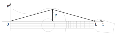
Imagine we have a tensioned guitar string of length $L$ . Suppose we only consider vibrations in one direction. That is, let $x$ denote the position along the string, let $t$ denote time, and let $y$ denote the displacement of the string from the rest position. See Figure $\PageIndex{1}$ .

Diagram of a vibrating string of length L over a faint guitar outline, pulled up into a sharp triangular peak at its midpoint, with an arrow there labelled y for displacement. — Figure $\PageIndex{1}$ : Vibrating string of length $L$ , $x$ is position, $y$ is displacement.

The equation that governs this setup is the so-called one-dimensional wave equation:

$y_{tt}=a^2 y_{xx}, \nonumber$

for some constant $a>0$ . The intuition is similar to the heat equation, replacing velocity with acceleration: the acceleration at a specific point is proportional to the second derivative of the shape of the string. In other words when the string is concave down then $u_{xx}$ is negative and the string wants to accelerate downwards, so $u_{tt}$ should be negative. And vice versa. The wave equation is an example of a hyperbolic PDE.

Assume that the ends of the string are fixed in place:

$y(0,t)=0 \quad\text{and}\quad y(L,t)=0. \nonumber$

Note that we have two conditions along the $x$ axis as there are two derivatives in the $x$ direction.

There are also two derivatives along the $t$ direction and hence we need two further conditions here. We need to know the initial position and the initial velocity of the string. That is, for some known functions $f(x)$ and $g(x)$ , we impose

$y(x,0)=f(x) \quad\text{and}\quad y_t(x,0)=g(x). \nonumber$

As the equation is again linear, superposition works just as it did for the heat equation. And again we will use separation of variables to find enough building-block solutions to get the overall solution. There is one change however. It will be easier to solve two separate problems and add their solutions.

The two problems we will solve are

$\label{wave:weq} \begin{array}{ll} w_{tt} = a^2 w_{xx}, & \\ w(0,t) = w(L,t) = 0, & \\ w(x,0) = 0 & \qquad \text{for } \; 0 < x < L, \\ w_t(x,0) = g(x) & \qquad \text{for } \; 0 < x < L, \end{array}$

(4.7.1)

and

$\label{wave:zeq} \begin{array}{ll} z_{tt} = a^2 z_{xx}, & \\ z(0,t) = z(L,t) = 0, & \\ z(x,0) = f(x) & \qquad \text{for } \; 0 < x < L, \\ z_t(x,0) = 0 & \qquad \text{for } \; 0 < x < L. \end{array}$

(4.7.2)

The principle of superposition implies that $y=w+z$ solves the wave equation and furthermore $y(x,0)=w(x,0)+z(x,0)=f(x)$ and $y_t(x,0)=w_t(x,0)+z_t(x,0)=g(x)$ . Hence, $y$ is a solution to

$\label{wave:yeq} \begin{array}{ll} y_{tt} = a^2 y_{xx}, & \\ y(0,t) = y(L,t) = 0, & \\ y(x,0) = f(x) & \qquad \text{for } \; 0 < x < L, \\ y_t(x,0) = g(x) & \qquad \text{for } \; 0 < x < L. \end{array}$

(4.7.3)

The reason for all this complexity is that superposition only works for homogeneous conditions such as $y(0,t)=y(L,t)=0$ , $y(x,0)=0$ , or $y_t(x,0)=0$ . Therefore, we will be able to use the idea of separation of variables to find many building-block solutions solving all the homogeneous conditions. We can then use them to construct a solution solving the remaining nonhomogeneous condition.

Let us start with (4.7.1). We try a solution of the form $w(x,t)=X(x)T(t)$ again. We plug into the wave equation to obtain

$X(x)T''(t)=a^2 X''(x)T(t). \nonumber$

Rewriting we get

$\dfrac{T''(t)}{a^2 T(t)}= \dfrac{X''(x)}{X(x)}. \nonumber$

Again, left hand side depends only on $t$ and the right hand side depends only on $x$ . Therefore, both equal a constant, which we will denote by $- \lambda$ .

$\dfrac{T''(t)}{a^2 T(t)}= - \lambda = \dfrac{X''(x)}{X(x)}. \nonumber$

We solve to get two ordinary differential equations

$\begin{align}\begin{aligned} X''(x)+ \lambda X(x) &=0, \\ T''(t)+ \lambda a^2T(t) &=0.\end{aligned}\end{align} \nonumber$

The conditions $0=w(0,t)=X(0)T(t)$ implies $X(0)=0$ and $w(L,t)=0$ implies that $X(L)=0$ . Therefore, the only nontrivial solutions for the first equation are when $\lambda = \lambda_n = \dfrac{n^2 \pi^2}{L^2}$ and they are

$X_n(x)= \sin \left( \dfrac{n \pi}{L}x \right). \nonumber$

The general solution for $T$ for this particular $\lambda_n$ is

$T_n(t)= A \cos \left( \dfrac{n \pi a}{L}t \right) + B \sin \left( \dfrac{n \pi a}{L}t \right). \nonumber$

We also have the condition that $w(x,0)=0$ or $X(x)T(0)=0$ . This implies that $T(0)=0$ , which in turn forces $A=0$ . It is convenient to pick $B= \dfrac{L}{n \pi a}$ (you will see why in a moment) and hence

$T_n(t)= \dfrac{L}{n \pi a} \sin \left( \dfrac{n \pi a}{L}t \right). \nonumber$

Our building-block solutions are

$w_n(x,t)= \dfrac{L}{n \pi a} \sin \left( \dfrac{n \pi }{L}x \right) \sin \left( \dfrac{n \pi a}{L}t \right). \nonumber$

We differentiate in $t$ , that is

$\dfrac{\partial w_n}{\partial t}(x,t)= \sin \left( \dfrac{n \pi }{L}x \right) \cos \left( \dfrac{n \pi a}{L}t \right). \nonumber$

Hence,

$\dfrac{\partial w_n}{\partial t}(x,0)= \sin \left( \dfrac{n \pi }{L}x \right). \nonumber$

We expand $g(x)$ in terms of these sines as

$g(x)= \sum_{n=1}^{\infty} b_n \sin \left( \dfrac{n \pi}{L}x \right). \nonumber$

Using superposition we can just write down the solution to (4.7.1) as a series

$w(x,t)= \sum_{n=1}^{\infty} b_n w_n(x,t) = \sum_{n=1}^{\infty} b_n \dfrac{L}{n \pi a} \sin \left( \dfrac{n \pi }{L}x \right) \sin \left( \dfrac{n \pi a}{L}t \right). \nonumber$

Similarly we proceed to solve (4.7.2). We again try $z(x,y)=X(x)T(t)$ . The procedure works exactly the same at first. We obtain

$\begin{align}\begin{aligned} X''(x)+ \lambda X(x) &=0, \\ T''(t)+ \lambda a^2T(t) &=0.\end{aligned}\end{align} \nonumber$

and the conditions $X(0)=0$ , $X(L)=0$ . So again $\lambda = \lambda_n = \dfrac{n^2 \pi^2}{L^2}$ and

$X_n(x)= \sin \left( \dfrac{n \pi}{L}x \right). \nonumber$

This time the condition on $T$ is $T'(0)=0$ . Thus we get that $B=0$ and we take

$T_n(t)= \cos \left( \dfrac{n \pi a}{L}t \right). \nonumber$

Our building-block solution will be

$z_n(x,t)= \sin \left( \dfrac{n \pi}{L}x \right) \cos \left( \dfrac{n \pi a}{L}t \right). \nonumber$

As $z_{n}(x,0)=\sin\left(\frac{n\pi}{L}x\right)$ , we expand $f(x)$ in terms of these sines as

$f(x)= \sum_{n=1}^{\infty}c_n \sin \left( \dfrac{n \pi}{L}x \right). \nonumber$

And we write down the solution to (4.7.2) as a series

$z(x,t)= \sum_{n=1}^{\infty}c_n z_n (x,t)= \sum_{n=1}^{\infty} c_n \sin \left( \dfrac{n \pi}{L}x \right) \cos \left( \dfrac{n \pi a}{L}t \right). \nonumber$

Putting these two solutions together, let us state the result as a theorem.

Note

Take the equation

$\label{wave:tyeq} \begin{array}{ll} y_{tt} = a^2 y_{xx}, & \\ y(0,t) = y(L,t) = 0, & \\ y(x,0) = f(x) & \qquad \text{for } \; 0 < x < L, \\ y_t(x,0) = g(x) & \qquad \text{for } \; 0 < x < L, \end{array}$

(4.7.4)

where

$f(x)= \sum_{n=1}^{\infty} c_n \sin \left( \dfrac{n \pi}{L}x \right), \nonumber$

and

$g(x)= \sum_{n=1}^{\infty} b_n \sin \left( \dfrac{n \pi}{L}x \right). \nonumber$

Then the solution $y(x,t)$ can be written as a sum of the solutions of (4.7.4) and (4.7.5). In other words,

$\begin{align}\begin{aligned} y(x,t) &= \sum_{n=1}^{\infty} b_n \dfrac{L}{n \pi a} \sin \left( \dfrac{n \pi}{L}x \right) \sin \left( \dfrac{n \pi a}{L}t \right) + c_n \sin \left( \dfrac{n \pi}{L}x \right) \cos \left( \dfrac{n \pi a}{L}t \right) \\ &= \sum_{n=1}^{\infty} \sin \left( \dfrac{n \pi}{L}x \right) \left[ b_n \dfrac{L}{n \pi a} \sin \left( \dfrac{n \pi a}{L}t \right) +c_n \cos \left( \dfrac{n \pi a}{L}t \right) \right].\end{aligned}\end{align} \nonumber$

Example 1

Let us try a simple example of a plucked string. Suppose that a string of length 2 is plucked in the middle such that it has the initial shape given in Figure $\PageIndex{2}$ . That is

$f(x)= \left\{ \begin{array}{cc} 0.1x & {\rm{if}}~ 0 \leq x \leq 1, \\ 0.1(2-x) & {\rm{if}}~ 1 < x \leq 2 \end{array} \right.. \nonumber$

Figure

\PageIndex{2}

: Initial shape of a plucked string from Example

\PageIndex{1}

The string starts at rest ( $g(x)=0$ ). Suppose that $a=1$ in the wave equation for simplicity. In other words, we wish to solve the problem:

$\begin{align}\begin{aligned} & y_{tt} = y_{xx}, \\ & y(0,t) = y(2,t)= 0, \\ & y(x,0) = f(x) \quad \text{and} \quad y_t(x,0)= 0.\end{aligned}\end{align} \nonumber$

We leave it to the reader to compute the sine series of $f(x)$ . The series will be

$f(x)= \sum_{n=1}^{\infty} \dfrac{0.8}{n^2 \pi^2} \sin \left( \dfrac{n \pi}{2} \right) \sin \left( \dfrac{n \pi}{2} x \right). \nonumber$

Note that $\sin \left( \dfrac{n \pi}{2} \right)$ is the sequence $1,0,-1,0,1,0,-1, \ldots$ for $n=1,2,3,4, \ldots$ . Therefore,

$f(x)= \dfrac{0.8}{ \pi^2} \sin \left( \dfrac{\pi}{2}x \right) - \dfrac{0.8}{9 \pi^2} \sin \left( \dfrac{3 \pi}{2}x \right) + \dfrac{0.8}{25 \pi^2} \sin \left( \dfrac{5 \pi}{2}x \right) - \cdots \nonumber$

The solution $y(x,t)$ is given by

$\begin{align}\begin{aligned} y(x,t) & = \sum_{n=1}^\infty \frac{0.8}{n^2 \pi^2} \sin \left( \frac{n \pi}{2} \right) \sin \left( \frac{n \pi}{2} x \right) \cos \left( \frac{n \pi}{2} t \right) \\ & = \sum_{m=1}^\infty \frac{0.8 {(-1)}^{m+1}}{{(2m-1)}^2 \pi^2} \sin \left( \frac{(2m-1) \pi}{2} x \right) \cos \left( \frac{(2m-1) \pi}{2} t \right) \\ & = \frac{0.8}{\pi^2} \sin \left( \frac{\pi}{2} x \right) \cos \left( \frac{\pi}{2} t \right) - \frac{0.8}{9 \pi^2} \sin \left( \frac{3 \pi}{2} x \right) \cos \left( \frac{3 \pi}{2} t \right) \\ & \hspace{20em} + \frac{0.8}{25 \pi^2} \sin \left( \frac{5 \pi}{2} x \right) \cos \left( \frac{5 \pi}{2} t \right) - \cdots \end{aligned}\end{align} \nonumber$

See Figure $\PageIndex{3}$ for a plot for $0 < t < 3$ . Notice that unlike the heat equation, the solution does not become "smoother," the "sharp edges" remain. We will see the reason for this behavior in the next section where we derive the solution to the wave equation in a different way.

Explore in 3D (opens in a new tab)

The displacement surface u(x, t) = cos(2 n t) sin(n x) for a standing mode of the string, time along the second axis. Contrast with the heat surface in 4.6: the wave carries its shape forever - the amplitude never decays, it only oscillates. Higher modes oscillate faster in both x and t.

Figure

\PageIndex{3}

: Shape of the plucked string for

0<t<3

Make sure you understand what the plot, such as the one in the figure, is telling you. For each fixed $t$ , you can think of the function $y(x,t)$ as just a function of $x$ . This function gives you the shape of the string at time $t$ . See Figure $\PageIndex{4}$ for plots of at $y$ as a function of $x$ at several different values of $t$ . On this plot you can see the sharp edges remaining much better.

Figure

\PageIndex{4}

: Plucked string for

t=0

t=0.4

t=0.8

, and

t=1.2

One thing to take away from all this is how a guitar sounds. Notice that the (angular) frequencies that come up in the solution are $n \frac{\pi a}{L}$ . That is, there is a certain base fundamental frequency $\frac{\pi a}{L}$ , and then we also get all the multiples of this frequency, which in music are called the overtones. Which overtones appear and with what amplitude is what musicians call the timbre of the note. Mathematicians usually call this the spectrum. Because all the frequencies are multiples of one frequency (the fundamental) we get a nice pleasing sound.

The fundamental frequency $\frac{\pi a}{L}$ increases as we decrease length $L$ . That is, if we place a finger on the fingerboard and then pluck a string we get a higher note. The constant $a$ is given by

$a = \sqrt{\frac{T}{\rho}}, \nonumber$

where

T

is tension and

\rho

is the linear density of the string. Tightening the string (turning the tuning peg on a guitar) increases

a

and hence produces a higher fundamental frequency (a higher note). On the other hand using a heavier string reduces

a

and produces a lower fundamental frequency (a lower note). A bass guitar has longer thicker strings, while a ukulele has short strings made of lighter material.

Something rather interesting is the almost symmetry between space and time. In its simplest form we see this symmetry in the solutions

$\sin \left( \frac{n \pi}{L} x \right) \sin \left( \frac{n \pi a}{L} t \right). \nonumber$

Except for the

a

, time and space are just the same.

In general, the solution for a fixed $x$ is a Fourier series in $t$ , for a fixed $t$ it is a Fourier series in $x$ , and the coefficients are related. If the shape $f(x)$ or the initial velocity have lots of corners, then the sound wave will have lots of corners. That is because the Fourier coefficients of the initial shape decay to zero (as $n \to \infty$ ) at the same rate as the Fourier coefficients of the wave in time (for some fixed $x$ ). So if you use a sharp object to pick the string, you get a sharper sound with lots of high frequency components, while if you use your thumb, you get a softer sound without so many high overtones. Similarly if you pluck close to the bridge, you are getting a pluck that looks more like the sawtooth, and you get an even sharper sound.

In fact, if you look at the formula for the solution, you see that for any fixed $x$ we get an almost arbitrary Fourier series in $t$ , everything except the constant term. You can essentially obtain any sound you want by plucking the string in just the right way. Of course we are considering an ideal string of no stiffness and no air resistance. Those variables clearly impact the sound as well.

Adapted from Differential Equations for Engineers by Jiří Lebl (https://www.jirka.org/diffyqs/), © Jiří Lebl, licensed under CC BY-SA 4.0. Changes were made. License: CC-BY-SA-4.0.