4.9 Steady State Temperature and the Laplacian

Suppose we have an insulated wire, a plate, or a 3-dimensional object. We apply certain fixed temperatures on the ends of the wire, the edges of the plate, or on all sides of the 3-dimensional object. We wish to find out what is the steady state temperature distribution. That is, we wish to know what will be the temperature after long enough period of time.

We are really looking for a solution to the heat equation that is not dependent on time. Let us first solve the problem in one space variable. We are looking for a function $u$ that satisfies

$u_{t} = k u_{x x},$

but such that $u sub t equals 0$ for all $x$ and $t$ . Hence, we are looking for a function of $x$ alone that satisfies $u sub x x equals 0$ . It is easy to solve this equation by integration and we see that $u = A x + B$ for some constants $A$ and $B$ .

Suppose we have an insulated wire, and we apply constant temperature $T sub 1$ at one end (say where $x equals 0$ ) and $T sub 2$ on the other end (at $x = L$ where $L$ is the length of the wire). Then our steady state solution is

$u (x) = \frac{T_{2} - T_{1}}{L} x + T_{1} .$

This solution agrees with our common sense intuition with how the heat should be distributed in the wire. So in one dimension, the steady state solutions are basically just straight lines.

Things are more complicated in two or more space dimensions. Let us restrict to two space dimensions for simplicity. The heat equation in two space variables is

$u_{t} = k (u_{x x} + u_{y y}),$

(4.9.1)

or more commonly written as $u_{t} = k Δ u$ or $u sub t equals k ∇ squared u$ . Here the $Δ$ and $∇ squared$ symbols mean $\frac{\partial^{2}}{\partial x^{2}} + \frac{\partial^{2}}{\partial y^{2}}$ . We will use $Δ$ from now on. The reason for using such a notation is that you can define $Δ$ to be the right thing for any number of space dimensions and then the heat equation is always $u_{t} = k Δ u$ . The operator $Δ$ is called the Laplacian.

OK, now that we have notation out of the way, let us see what does an equation for the steady state solution look like. We are looking for a solution to Equation (4.9.1) that does not depend on $t$ , or in other words $u sub t equals 0$ . Hence we are looking for a function $u (x, y)$ such that

$Δ u = u_{x x} + u_{y y} = 0 .$

This equation is called the Laplace equationto the power 1. Solutions to the Laplace equation are called harmonic functions and have many nice properties and applications far beyond the steady state heat problem.

Harmonic functions in two variables are no longer just linear (plane graphs). For example, you can check that the functions $x^{2} - y^{2}$ and $x y$ are harmonic. However, if you remember your multi-variable calculus we note that if $u_{x x}$ is positive, $u$ is concave up in the $x$ direction, then $u_{y y}$ must be negative and $u$ must be concave down in the $y$ direction. Therefore, a harmonic function can never have any “hilltop” or “valley” on the graph. This observation is consistent with our intuitive idea of steady state heat distribution; the hottest or coldest spot will not be inside.

Commonly the Laplace equation is part of a so-called Dirichlet problemsquared. That is, we have a region in the $x y$ -plane and we specify certain values along the boundaries of the region. We then try to find a solution $u$ defined on this region such that $u$ agrees with the values we specified on the boundary.

For simplicity, we consider a rectangular region. Also for simplicity we specify boundary values to be zero at 3 of the four edges and only specify an arbitrary function at one edge. As we still have the principle of superposition, we can use this simpler solution to derive the general solution for arbitrary boundary values by solving 4 different problems, one for each edge, and adding those solutions together. This setup is left as an exercise.

We wish to solve the following problem. Let $h$ and $w$ be the height and width of our rectangle, with one corner at the origin and lying in the first quadrant.

$\begin{matrix} Δ u = 0, \\ u (0, y) = 0 for 0 < y < h, \\ u (x, h) = 0 for 0 < x < w, \\ u (w, y) = 0 for 0 < y < h, \\ u (x, 0) = f (x) for 0 < x < w . \end{matrix}$

(4.9.2)

Diagram of a rectangle with corners (0,0), (w,0), (0,h) and (w,h) and delta u equals 0 inside; the left, right and top edges are labelled u equals 0 and the bottom edge u equals f of x. — Figure $1$

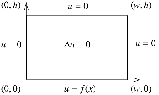
The method we apply is separation of variables. Again, we will come up with enough building-block solutions satisfying all the homogeneous boundary conditions (all conditions except (4.9.6)). We notice that superposition still works for the equation and all the homogeneous conditions. Therefore, we can use the Fourier series for $f (x)$ to solve the problem as before.

We try $u (x, y) = X (x) Y (y)$ . We plug $u$ into the equation to get

$X^{″} Y + X Y^{″} = 0 .$

We put the $X$ s on one side and the $Y$ s on the other to get

$- \frac{X^{″}}{X} = \frac{Y^{″}}{Y} .$

The left hand side only depends on $x$ and the right hand side only depends on $y$ . Therefore, there is some constant $λ$ such that $λ = \frac{- X^{″}}{X} = \frac{Y^{″}}{Y}$ . And we get two equations

$X^{″} + λ X = 0, Y^{″} - λ Y = 0 .$

Furthermore, the homogeneous boundary conditions imply that $X (0) = X (w) = 0$ and $Y open parenthesis h close parenthesis equals 0$ . Taking the equation for $X$ we have already seen that we have a nontrivial solution if and only if $λ = λ_{n} = \frac{n^{2} π^{2}}{w^{2}}$ and the solution is a multiple of

$X_{n} (x) = \sin (\frac{n π}{w} x) .$

For these given $λ_{n}$ , the general solution for $Y$ (one for each $n$ ) is

$Y_{n} (y) = A_{n} \cosh (\frac{n π}{w} y) + B_{n} \sinh (\frac{n π}{w} y) .$

(4.9.7)

We only have one condition on $Y_{n}$ and hence we can pick one of $A_{n}$ or $B_{n}$ to be something convenient. It will be useful to have $Y sub n open parenthesis 0 close parenthesis equals 1$ , so we let $A sub n equals 1$ . Setting $Y sub n open parenthesis h close parenthesis equals 0$ and solving for $B_{n}$ we get that

$B_{n} = \frac{- \cosh (\frac{n π h}{w})}{\sinh (\frac{n π h}{w})} .$

After we plug the $A_{n}$ and $B_{n}$ we into (4.9.7) and simplify, we find

$Y_{n} (y) = \frac{\sinh (\frac{n π (h - y)}{w})}{\sinh (\frac{n π h}{w})} .$

We define $u_{n} (x, y) = X_{n} (x) Y_{n} (y)$ . And note that $u_{n}$ satisfies (4.9.2) - (4.9.5).

Observe that

$u_{n} (x, 0) = X_{n} (x) Y_{n} (0) = \sin (\frac{n π}{w} x) .$

Suppose

$f (x) = \sum_{n = 1}^{\infty} b_{n} \sin (\frac{n π x}{w}) .$

Then we get a solution of (4.9.2) - (4.9.6) of the following form.

$u (x, y) = \sum_{n = 1}^{\infty} b_{n} u_{n} (x, y) = \sum_{n = 1}^{\infty} b_{n} \sin (\frac{n π}{w} x) (\frac{\sinh (\frac{n π (h - y)}{w})}{\sinh (\frac{n π h}{w})}) .$

As $u_{n}$ satisfies Equation (4.9.2) - (4.9.5) and any linear combination (finite or infinite) of $u_{n}$ must also satisfy (4.9.2) - (4.9.5), we see that $u$ must satisfy Equations (4.9.2) - (4.9.5). By plugging in $y equals 0$ it is easy to see that $u$ satisfies (4.9.6) as well.

Example 1

Suppose that we take $w = h = π$ and we let $f (x) = π$ . We compute the sine series for the function $π$ (we will get the square wave). We find that for $0 less than x less than π$ we have

$f (x) = \sum_{\underset{n o d d}{n = 1}}^{\infty} \frac{4}{n} \sin (n x) .$

Therefore the solution $u (x, y)$ , see Figure $2$ , to the corresponding Dirichlet problem is given as

$u (x, y) = \sum_{\underset{n o d d}{n = 1}}^{\infty} \frac{4}{n} \sin (n x) (\frac{\sinh (n (π - y))}{\sinh (n π)}) .$

Figure

2

: Steady state temperature of a square plate, three sides held at zero and one side held at

π

This scenario corresponds to the steady state temperature on a square plate of width $π$ with 3 sides held at 0 degrees and one side held at $π$ degrees. If we have arbitrary initial data on all sides, then we solve four problems, each using one piece of nonhomogeneous data. Then we use the principle of superposition to add up all four solutions to have a solution to the original problem.

A different way to visualize solutions of the Laplace equation is to take a wire and bend it so that it corresponds to the graph of the temperature above the boundary of your region. Cut a rubber sheet in the shape of your region—a square in our case—and stretch it fixing the edges of the sheet to the wire. The rubber sheet is a good approximation of the graph of the solution to the Laplace equation with the given boundary data.

Footnotes

[1] Named after the French mathematician Pierre-Simon, marquis de Laplace (1749–1827).

[2] Named after the German mathematician Johann Peter Gustav Lejeune Dirichlet (1805–1859).

Adapted from Differential Equations for Engineers by Jiří Lebl (Oklahoma State University), hosted on LibreTexts (math.libretexts.org) and licensed under CC BY-SA 4.0. Changes were made. License: CC-BY-SA-4.0.