Differential Equations for EngineersXYZ Homework Edition

⇩ Download ▾

4.10 Dirichlet Problem in the Circle and the Poisson Kernel

Laplace in Polar Coordinates

A more natural setting for the Laplace equation Δu=0\Delta u=0 is the circle rather than the square. On the other hand, what makes the problem somewhat more difficult is that we need polar coordinates.

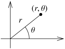
Diagram of polar coordinates: a ray from the origin into the first quadrant ending at a point labelled (r, theta), the ray labelled r and an arc marking the angle theta.
Figure 1

Recall that the polar coordinates for the (x,y)(x,y)-plane are (r,θ)(r, \theta ):

x = r cos θ , y = r sin θ , x= r \cos \theta, ~~~~ y= r \sin \theta, \nonumber

where r≥0r \geq 0 and −π<θ<π- \pi < \theta < \pi. So (x,y)(x,y) is distance rr from the origin at angle θ\theta from the positive xx-axis.

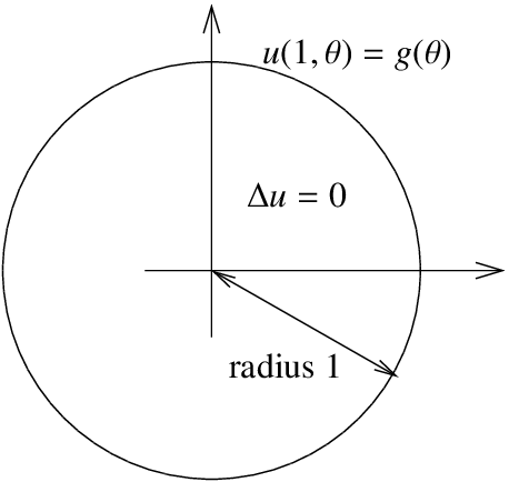
Diagram of the Dirichlet problem in a disc: a circle centred at the origin with delta u equals 0 inside, an arrow marking radius 1, and the rim labelled u of 1 and theta equals g of theta.
Figure 2

Now that we know our coordinates, let us give the problem we wish to solve. We have a circular region of radius 1, and we are interested in the Dirichlet problem for the Laplace equation for this region. Let u(r,θ)u(r, \theta ) denote the temperature at the point (r,θ)(r, \theta ) in polar coordinates. We have the problem:

Δ u = 0 , f o r r < 1 , u ( 1 , θ ) = g ( θ ) , f o r π < θ ≤ π . \begin{align} \Delta u &=0, & {\rm{for~}} r<1, \label{eq:2} \\ u(1, \theta ) &=g( \theta), &{\rm{for~}} \pi < \theta \leq \pi. \end{align} \nonumber

(4.10.1)

The first issue we face is that we do not know what the Laplacian is in polar coordinates. Normally we would find uxxu_{xx} and uyyu_{yy} in terms of the derivatives in rr and θ\theta. We would need to solve for rr and θ\theta in terms of xx and yy. While this is certainly possible, it happens to be more convenient to work in reverse. Let us instead compute derivatives in rr and θ\theta in terms of derivatives in xx and yy and then solve. The computations are easier this way. First

x r = cos θ , x θ = − r sin θ , y r = sin θ , y θ = r cos θ . \begin{align}\begin{aligned} x_r &= \cos \theta, &x_{\theta}= -r \sin \theta, \\ y_{r} &= \sin \theta, & y_{\theta}= r \cos \theta. \end{aligned}\end{align} \nonumber

Next by chain rule we obtain

u r = u x x r + u y y r = cos ( θ ) u x + sin ( θ ) u y , u r r = cos ( θ ) ( u x x x r + u x y y r ) + sin ( θ ) ( u y x x r + u y y y r ) = cos 2 ( θ ) u x x + 2 cos ( θ ) sin ( θ ) u x y + sin 2 ( θ ) u y y . \begin{align}\begin{aligned} u_r &=u_xx_{r}+u_yy_{r}= \cos(\theta)u_x + \sin(\theta)u_y, \\ u_{rr} &= \cos(\theta)(u_{xx}x_r+u_{xy}y_r)+ \sin(\theta)(u_{yx}x_r+u_{yy}y_r) \\ &= \cos^2(\theta)u_{xx}+2 \cos(\theta) \sin(\theta)u_{xy}+ \sin^2(\theta)u_{yy}.\end{aligned}\end{align} \nonumber

Similarly for the θ\theta derivative. Note that we have to use product rule for the second derivative.

u θ = u x x θ + u y y θ = − r sin ( θ ) u x + r cos ( θ ) u y , u θ θ = − r cos ( θ ) ( u x ) − r sin ( θ ) ( u x x x θ + u x y y θ ) − r sin ( θ ) ( u y ) + r cos ( θ ) ( u y x x θ + u y y y θ ) = − r cos ( θ ) u x − r sin ( θ ) u y + r 2 sin 2 ( θ ) u x x − r 2 2 sin ( θ ) cos ( θ ) u x y + r 2 cos 2 ( θ ) u y y . \begin{align}\begin{aligned} u_{\theta} &=u_xx_{\theta}+u_yy_{\theta}= -r \sin(\theta)u_x + r \cos(\theta)u_y, \\ u_{\theta \theta} &= -r \cos(\theta)(u_x)- r \sin(\theta)(u_{xx}x_{\theta}+u_{xy}y_{\theta})-r \sin(\theta)(u_y)+r \cos(\theta)(u_{yx}x_{\theta}+u_{yy}y_{\theta}) \\ &= -r \cos(\theta)u_{x}-r \sin(\theta)u_y+r^2 \sin^2(\theta)u_{xx}-r^2 2 \sin(\theta) \cos(\theta) u_{xy}+r^2 \cos^2(\theta)u_{yy}.\end{aligned}\end{align} \nonumber

Let us now try to solve for uxx+uyyu_{xx}+u_{yy}. We start with 1r2uθθ\frac{1}{r^2}u_{\theta \theta} to get rid of those pesky r2r^2. If we add urru_{rr} and use the fact that cos2(θ)+sin2(θ)=1\cos^2(\theta)+ \sin^2(\theta)=1, we get

1 r 2 u θ θ + u r r = u x x + u y y − 1 r cos ( θ ) u x − 1 r sin ( θ ) u y . \frac{1}{r^2}u_{\theta \theta} +u_{rr}=u_{xx}+u_{yy}- \frac{1}{r} \cos(\theta)u_x- \frac{1}{r} \sin(\theta)u_y. \nonumber

We’re not quite there yet, but all we are lacking is 1rur\frac{1}{r}u_r. Adding it we obtain the Laplacian in polar coordinates:

1 r 2 u θ θ + 1 r u r + u r r = u x x + u y y = Δ u . \frac{1}{r^2}u_{\theta \theta}+ \frac{1}{r}u_{r}+u_{rr}=u_{xx}+u_{yy}= \Delta u. \nonumber

Notice that the Laplacian in polar coordinates no longer has constant coefficients.

Series Solution

Let us separate variables as usual. That is let us try u(r,θ)=R(r)Θ(θ)u(r, \theta)=R(r) \Theta ( \theta). Then

0 = Δ u = 1 r 2 R Θ ″ + 1 r R ′ Θ + R ″ Θ . 0= \Delta u=\frac{1}{r^2}R \Theta''+ \frac{1}{r}R' \Theta+R'' \Theta. \nonumber

Let us put RR on one side and Θ\Theta on the other and conclude that both sides must be constant.

1 r 2 R Θ ″ = − ( 1 r R ′ + R ″ ) Θ . Θ ″ Θ = − r R ′ + r 2 R ″ R + − λ . \begin{align}\begin{aligned} \frac{1}{r^2}R \Theta'' &= - \left( \frac{1}{r}R'+R'' \right) \Theta. \\ \frac{ \Theta''}{ \Theta} &= - \frac{rR'+r^2R''}{R} + - \lambda.\end{aligned}\end{align} \nonumber

We get two equations:

Θ ″ + λ Θ = 0 , r 2 R ″ + r R ′ − λ R = 0 . \begin{align}\begin{aligned} \Theta''+\lambda \Theta &=0, \\ r^2R''+rR'- \lambda R &=0.\end{aligned}\end{align} \nonumber

Let us first focus on Θ\Theta. We know that u(r,θ)u(r, \theta) ought to be 2π2 \pi-periodic in θ\theta, that is, u(r,θ)=u(r,θ+2π)u(r, \theta)=u(r, \theta +2 \pi). Therefore, the solution to Θ″+λΘ=0\Theta''+\lambda \Theta=0 must be 2π2 \pi-periodic. We have seen such a problem in Example 4.1.5. We conclude that λ=n2\lambda=n^2 for a nonnegative integer n=0,1,2,3,...n=0,1,2,3,.... The equation becomes Θ″+n2Θ=0\Theta''+n^2 \Theta=0. When n=0n=0 the equation is just Θ″=0\Theta''=0, so we have the general solution Aθ+BA \theta+B. As Θ\Theta is periodic, A=0A=0. For convenience let us write this solution as

Θ 0 = a 0 2 \Theta_0=\frac{a_0}{2} \nonumber

for some constant a0a_0. For positive nn, the solution to Θ″+n2Θ=0\Theta''+n^2 \Theta=0 is

Θ n = a n cos ( n θ ) + b n sin ( n θ ) , \Theta_n=a_n \cos(n \theta)+b_n \sin(n \theta), \nonumber

for some constants ana_n and bnb_n.

Next, we consider the equation for RR,

r 2 R ″ + r R ′ − n 2 R = 0 . r^2R''+rR'-n^2R=0. \nonumber

This equation has appeared in exercises before—we solved it in Exercise 2.E.2.1.6 and Exercise 2.E.1.7. The idea is to try a solution rsr^s and if that does not work out try a solution of the form rslnrr^s \ln r. When n=0n=0 we obtain

R 0 = A r 0 + B r 0 ln r = A + B ln r , R_0=Ar^0+Br^0 \ln r=A+B \ln r, \nonumber

and if n>0n>0, we get

R n = A r n + B r − n . R_n=Ar^n+Br^{-n}. \nonumber

The function u(r,θ)u(r, \theta) must be finite at the origin, that is, when r=0r=0. Therefore, B=0B=0 in both cases. Let us set A=1A=1 in both cases as well, the constants in Θn\Theta_n will pick up the slack so we do not lose anything. Therefore let

R 0 = 1 , and R n = r n . R_0=1,\quad\text{and}\quad R_n=r^n. \nonumber

Hence our building block solutions are

u 0 ( r , θ ) = a 0 2 , u n ( r , θ ) = a n r n cos ( n θ ) + b n r n sin ( n θ ) . u_0(r, \theta)= \frac{a_0}{2},\quad u_n(r, \theta)=a_n r^n \cos(n \theta)+b_n r^n \sin(n \theta). \nonumber

Putting everything together our solution is:

u ( r , θ ) = a 0 2 + ∑ n = 1 ∞ a n r n cos ( n θ ) + b n r n sin ( n θ ) . u(r, \theta)= \frac{a_0}{2}+ \sum_{n=1}^{\infty}a_n r^n \cos(n \theta)+b_n r^n \sin(n \theta). \nonumber

We look at the boundary condition in (4.10.1),

g ( θ ) = u ( 1 , θ ) = a 0 2 + ∑ n = 1 ∞ a n cos ( n θ ) + b n sin ( n θ ) . g(\theta)=u(1, \theta)= \frac{a_0}{2}+ \sum_{n=1}^{\infty}a_n \cos(n \theta)+b_n \sin(n \theta). \nonumber

Therefore, the solution (4.10.1) is to expand g(θ)g(\theta), which is a 2π2 \pi-periodic function as a Fourier series, and then the nthn^{\text{th}} coordinate is multiplied by rnr^n. In other words, to compute ana^n and bnb^n from the formula we can, as usual, compute

a n = 1 π ∫ π − π g ( θ ) cos ( n θ ) d θ , and b n = 1 π ∫ π − π g ( θ ) sin ( n θ ) d θ . a_n= \frac{1}{ \pi} \int_{ \pi}^{- \pi} g(\theta) \cos(n \theta)d \theta, \quad\text{and}\quad b_n= \frac{1}{ \pi} \int_{ \pi}^{- \pi} g(\theta) \sin(n \theta)d \theta. \nonumber

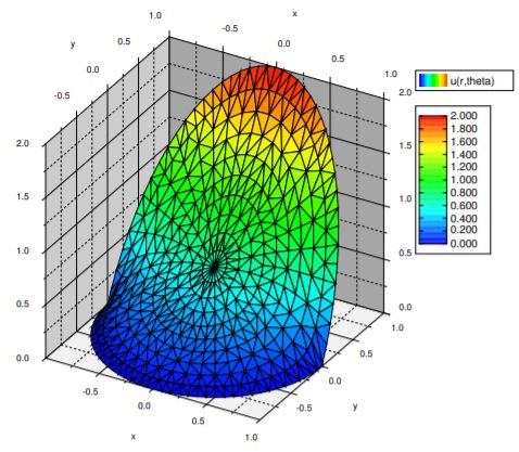
We now simply write the solution (see Figure 4) by multiplying by rnr^n in the right places.

u ( r , θ ) = 2 π + r sin ( θ ) + ∑ n = 1 ∞ − 4 r 2 n π ( 4 n 2 − 1 ) cos ( 2 n θ ) . u(r, \theta)= \frac{2}{\pi}+ r\sin(\theta)+ \sum_{n=1}^{\infty} \frac{-4r^{2n}}{\pi (4n^2-1)} \cos(2n \theta). \nonumber

Three-dimensional surface over the unit disc, height 0 to 2. Half the rim is held at 0 and lies low; over the other half the surface swells into a dome reaching 2 at the rim, with the centre only about 0.6 to 0.7.
Figure 4: The solution of the Dirichlet problem with boundary data 00 for y<0y<0 and 2y2y for y>0y>0.

Poisson Kernel

There is another way to solve the Dirichlet problem with the help of an integral kernel. That is, we will find a function P(r,θ,α)P(r,\theta,\alpha) called the Poisson kernel1 such that

u ( r , θ ) = 1 2 π ∫ − π π P ( r , θ , α ) g ( α ) d α . u(r,\theta)= \frac{1}{2\pi} \int_{-\pi}^{\pi}P(r,\theta,\alpha)g(\alpha)d\alpha. \nonumber

While the integral will generally not be solvable analytically, it can be evaluated numerically. In fact, unless the boundary data is given as a Fourier series already, it will be much easier to numerically evaluate this formula as there is only one integral to evaluate.

The formula also has theoretical applications. For instance, as P(r,θ,α)P(r,\theta,\alpha) will have infinitely many derivatives, then via differentiating under the integral we find that the solution u(r,θ)u(r,\theta) has infinitely many derivatives, at least when inside the circle, r<1r<1. By infinitely many derivatives what you should think of is that u(r,θ)u(r,\theta) has “no corners” and all of its partial derivatives exist too and also have “no corners”.

We will compute the formula for P(r,θ,α)P(r,\theta,\alpha) from the series solution, and this idea can be applied anytime you have a convenient series solution where the coefficients are obtained via integration. Hence you can apply this reasoning to obtain such integral kernels for other equations, such as the heat equation. The computation is long and tedious, but not overly difficult. Since the ideas are often applied in similar contexts, it is good to understand how this computation works.

What we do is start with the series solution and replace the coefficients with the integrals that compute them. Then we try to write everything as a single integral. We must use a different dummy variable for the integration and hence we use α\alpha instead of θ\theta.

u ( r , θ ) = a 0 2 + ∑ n = 1 ∞ a n r n cos ( n θ ) + b n r n sin ( n θ ) = ( 1 2 π ∫ − π π g ( α ) d α ) ⏟ a 0 2 + ∑ n = 1 ∞ ( 1 π ∫ − π π g ( α ) cos ( n α ) d α ) ⏟ a n r n cos ( n θ ) + ( 1 π ∫ − π π g ( α ) sin ( n α ) d α ) ⏟ b n r n sin ( n θ ) = 1 2 π ∫ − π π ( g ( α ) + 2 ∑ n = 1 ∞ g ( α ) cos ( n α ) r n cos ( n θ ) + g ( α ) sin ( n α ) r n sin ( n θ ) ) d α = 1 2 π ∫ − π π ( 1 + 2 ∑ n = 1 ∞ r n ( cos ( n α ) cos ( n θ ) + sin ( n α ) sin ( n θ ) ) ) ⏟ P ( r , θ , α ) g ( α ) d α \begin{align}\begin{aligned} u(r,\theta )&=\frac{a_{0}}{2}+\sum\limits_{n=1}^\infty a_{n}r^{n}\cos (n\theta )+b_{n}r^{n}\sin (n\theta ) \\ &=\underset{\frac{a_{0}}{2}}{\underbrace{\left(\frac{1}{2\pi}\int_{-\pi}^{\pi}g(\alpha )d\alpha\right)}}+\sum\limits_{n=1}^\infty \underset{a_{n}}{\underbrace{\left(\frac{1}{\pi}\int_{-\pi}^{\pi}g(\alpha)\cos (n\alpha )d\alpha\right)}}r^{n}\cos (n\theta) \\ &+\underset{b_{n}}{\underbrace{\left(\frac{1}{\pi}\int_{-\pi}^{\pi}g(\alpha)\sin (n\alpha)d\alpha\right)}}r^{n}\sin (n\theta ) \\ &=\frac{1}{2\pi}\int_{-\pi}^{\pi}\left(g(\alpha)+2\sum\limits_{n=1}^\infty g(\alpha)\cos (n\alpha)r^{n}\cos (n\theta )+g(\alpha )\sin (n\alpha )r^{n}\sin (n\theta )\right) d\alpha \\ &=\frac{1}{2\pi}\int_{-\pi}^{\pi}\underset{P(r,\theta,\alpha )}{\underbrace{\left( 1+2\sum\limits_{n=1}^\infty r^{n}\left(\cos (n\alpha )\cos (n\theta )+\sin (n\alpha )\sin (n\theta )\right)\right)}}g(\alpha )d\alpha \end{aligned}\end{align} \nonumber

OK, so we have what we wanted, the expression in the parentheses is the Poisson kernel, P(r,θ,α)P(r,\theta,\alpha). However, we can do a lot better. It is still given as a series, and we would really like to have a nice simple expression for it. We must work a little harder. The trick is to rewrite everything in terms of complex exponentials. Let us work just on the kernel.

P ( r , θ , α ) = 1 + 2 ∑ n = 1 ∞ r n ( cos ( n α ) cos ( n θ ) + sin ( n α ) sin ( n θ ) ) = 1 + 2 ∑ n = 1 ∞ r n cos ( n ( θ − α ) ) = 1 + 2 ∑ n = 1 ∞ r n ( e i n ( θ − α ) + e − i n ( θ − α ) ) = 1 + ∑ n = 1 ∞ ( r e i ( θ − α ) ) n + ∑ n = 1 ∞ ( r e − i ( θ − α ) ) n . \begin{align}\begin{aligned} P(r,\theta,\alpha) &=1+2\sum_{n=1}^{\infty}r^n(\cos(n\alpha)\cos(n\theta)+ \sin(n\alpha)\sin(n\theta)) \\ &= 1+2\sum_{n=1}^{\infty}r^n \cos(n(\theta- \alpha)) \\ &= 1+2\sum_{n=1}^{\infty}r^n(e^{in(\theta-\alpha)}+e^{-in(\theta-\alpha)}) \\ &= 1+\sum_{n=1}^{\infty}(re^{i(\theta-\alpha)})^n+\sum_{n=1}^{\infty}(re^{-i(\theta-\alpha)})^n.\end{aligned}\end{align} \nonumber

In the above expression we recognize the geometric series. That is, recall from calculus that as long as |z|<1|z|<1, then

∑ n = 1 ∞ z n = z 1 − z . \sum_{n=1}^{\infty}z^n= \frac{z}{1-z}. \nonumber

Note that nn starts at 11 and that is why we have the zz in the numerator. It is the standard geometric series multiplied by zz. Let us continue with the computation.

P ( r , θ , α ) = 1 + ∑ n = 1 ∞ ( r e i ( θ − α ) ) n + ∑ n = 1 ∞ ( r e − i ( θ − α ) ) n = 1 + r e i ( θ − α ) 1 − r e i ( θ − α ) + r e − i ( θ − α ) 1 − r e − i ( θ − α ) = ( 1 − r e i ( θ − α ) ) ( 1 − r e − i ( θ − α ) ) + ( 1 − r e − i ( θ − α ) ) r e i ( θ − α ) + ( 1 − r e i ( θ − α ) ) r e − i ( θ − α ) ( 1 − r e i ( θ − α ) ) ( 1 − r e − i ( θ − α ) ) = 1 − r 2 1 − r e i ( θ − α ) − r e − i ( θ − α ) + r 2 = 1 − r 2 1 − 2 r cos ( θ − α ) + r 2 . \begin{align}\begin{aligned} P(r,\theta,\alpha) &=1+\sum_{n=1}^{\infty}(re^{i(\theta-\alpha)})^n+\sum_{n=1}^{\infty}(re^{-i(\theta-\alpha)})^n \\ &= 1+ \frac{re^{i(\theta-\alpha)}}{1-re^{i(\theta-\alpha)}}+ \frac{re^{-i(\theta-\alpha)}}{1-re^{-i(\theta-\alpha)}} \\ &=\frac{(1-re^{i(\theta-\alpha)})(1-re^{-i(\theta-\alpha)})+(1-re^{-i(\theta-\alpha)})re^{ i(\theta-\alpha)}+(1-re^{i(\theta-\alpha)})re^{ - i(\theta-\alpha)}}{(1-re^{i(\theta-\alpha)})(1-re^{-i(\theta-\alpha)})} \\ &= \frac{1-r^2}{1-re^{i(\theta-\alpha)}-re^{-i(\theta-\alpha)}+r^2} \\ &= \frac{1-r^2}{1-2r\cos(\theta-\alpha)+r^2}.\end{aligned}\end{align} \nonumber

Now that’s a formula we can live with. The solution to the Dirichlet problem using the Poisson kernel is

u ( r , θ ) = 1 2 π ∫ − π π 1 − r 2 1 − 2 r cos ( θ − α ) + r 2 g ( α ) d α . u(r, \theta)= \frac{1}{2\pi} \int_{-\pi}^{\pi} \frac{1-r^2}{1-2r\cos(\theta-\alpha)+r^2}g(\alpha)d\alpha. \nonumber

Sometimes the formula for the Poisson kernel is given together with the constant 12π\frac{1}{2\pi}, in which case we should of course not leave it in front of the integral. Also, often the limits of the integral are given as 00 to 2π2\pi; everything inside is 2π2\pi-periodic in α\alpha, so this does not change the integral.

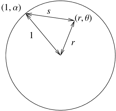
Let us not leave the Poisson kernel without explaining its geometric meaning. Let ss be the distance from (r,θ)(r,\theta) to (1,α)(1,\alpha). You may recall from calculus that this distance ss in polar coordinates is given precisely by the square root of 1−2rcos(θ−α)+r21-2r\cos(\theta-\alpha)+r^2. That is, the Poisson kernel is really the formula

1 − r 2 s 2 . \frac{1-r^2}{s^2}. \nonumber

Diagram of a circle with a radius labelled 1 drawn to a rim point (1, alpha), a segment labelled r from the centre to an interior point (r, theta), and a segment s joining those two points.
Figure 5

One final note we make about the formula is to note that it is really a weighted average of the boundary values. First let us look at what happens at the origin, that is when r=0r=0.

u ( 0 , 0 ) = 1 2 π ∫ − π π 1 − 0 2 1 − 2 ( 0 ) cos ( θ − α ) + 0 2 g ( α ) d α = 1 2 π ∫ − π π g ( α ) d α . \begin{align}\begin{aligned} u(0,0) &= \frac{1}{2\pi} \int_{-\pi}^{\pi} \frac{1-0^2}{1-2(0)\cos(\theta-\alpha)+0^2}g(\alpha)d\alpha \\ &= \frac{1}{2\pi} \int_{-\pi}^{\pi} g(\alpha)d\alpha. \end{aligned}\end{align} \nonumber

So u(0,0)u(0,0) is precisely the average value of g(θ)g(\theta) and therefore the average value of uu on the boundary. This is a general feature of harmonic functions, the value at some point pp is equal to the average of the values on a circle centered at pp.

What the formula says is that the value of the solution at any point in the circle is a weighted average of the boundary data g(θ)g(\theta). The kernel is bigger when (r,θ)(r,\theta) is closer to (1,α)(1,\alpha). Therefore when computing u(r,θ)u(r,\theta) we give more weight to the values g(α)g(\alpha) when (1,α)(1,\alpha) is closer to (r,θ)(r,\theta) and less weight to the values g(θ)g(\theta) when (1,α)(1,\alpha) far from (r,θ)(r,\theta).

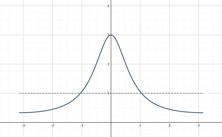
Interactive figureThe Poisson kernel as a weighted average of the boundary dataDrag the Radius r of the point in the disc slider from 0 to 0.6.
A hump rises above a horizontal dashed line in the middle of the frame and sinks below it toward both edges, so boundary points near the centre are weighted heavily while those on the far side barely count. Sliding the radius in to zero flattens the hump onto the dashed line — every boundary point weighted equally. Sliding it outward sharpens the hump into a tall narrow spike while the far side sags closer to the axis; the area underneath never changes. Adjustable parameter: Radius r of the point in the disc (r) = 0.5. Viewing window: x from -3.8 to 3.8, y from -0.5 to 4.2.
XYZ Graph · viewer build 5edf91b
The kernel P(r, θ, α) = (1 − r²)/(1 − 2r cos(θ − α) + r²) plotted against the boundary angle α, for an observation angle θ = 0: the horizontal axis says which boundary point, the vertical axis says how much weight it gets. Drag r out from the centre. At r = 0 the kernel lies flat on the dashed line at 1 — that is exactly the mean value property just proved, u(0, 0) = the average of g. By r = 0.6 it is a spike of height 4 over α = 0 while the far side of the circle has sunk to 0.25. The area underneath never changes, so this is re-weighting, not growth — which is also why a fast-wiggling boundary condition like cos(10θ) is felt at the boundary and dies before the middle of the disc.

Footnotes

[1] Named for the French mathematician Siméon Denis Poisson (1781 – 1840).

Adapted from Differential Equations for Engineers by Jiří Lebl (https://www.jirka.org/diffyqs/), © Jiří Lebl, licensed under CC BY-SA 4.0. Changes were made. License: CC-BY-SA-4.0.

These eBooks are a prerelease and are not yet certified conformant with WCAG 2.1 AA or any other accessibility standard. Every page is built against an automated accessibility gate, and our target for the published editions is WCAG 2.2 Level AA. If something is unusable, please tell us.