4.10 Dirichlet Problem in the Circle and the Poisson Kernel

Laplace in Polar Coordinates

A more natural setting for the Laplace equation $Δ u equals 0$ is the circle rather than the square. On the other hand, what makes the problem somewhat more difficult is that we need polar coordinates.

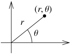
Diagram of polar coordinates: a ray from the origin into the first quadrant ending at a point labelled (r, theta), the ray labelled r and an arc marking the angle theta. — Figure $1$

Recall that the polar coordinates for the $(x, y)$ -plane are $(r, θ)$ :

$x = r \cos θ, y = r \sin θ,$

where $r greater than or equal to 0$ and $- π < θ < π$ . So $(x, y)$ is distance $r$ from the origin at angle $θ$ from the positive $x$ -axis.

Diagram of the Dirichlet problem in a disc: a circle centred at the origin with delta u equals 0 inside, an arrow marking radius 1, and the rim labelled u of 1 and theta equals g of theta. — Figure $2$

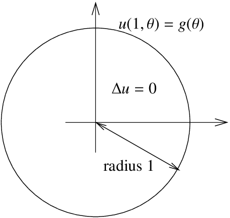
Now that we know our coordinates, let us give the problem we wish to solve. We have a circular region of radius 1, and we are interested in the Dirichlet problem for the Laplace equation for this region. Let $u (r, θ)$ denote the temperature at the point $(r, θ)$ in polar coordinates. We have the problem:

$\begin{matrix} Δ u = 0, f o r r < 1, \\ u (1, θ) = g (θ), f o r π < θ \leq π . \end{matrix}$

(4.10.1)

The first issue we face is that we do not know what the Laplacian is in polar coordinates. Normally we would find $u_{x x}$ and $u_{y y}$ in terms of the derivatives in $r$ and $θ$ . We would need to solve for $r$ and $θ$ in terms of $x$ and $y$ . While this is certainly possible, it happens to be more convenient to work in reverse. Let us instead compute derivatives in $r$ and $θ$ in terms of derivatives in $x$ and $y$ and then solve. The computations are easier this way. First

$\begin{matrix} x_{r} = \cos θ, x_{θ} = - r \sin θ, \\ y_{r} = \sin θ, y_{θ} = r \cos θ . \end{matrix}$

Next by chain rule we obtain

$\begin{matrix} u_{r} = u_{x} x_{r} + u_{y} y_{r} = \cos (θ) u_{x} + \sin (θ) u_{y}, \\ u_{r r} = \cos (θ) (u_{x x} x_{r} + u_{x y} y_{r}) + \sin (θ) (u_{y x} x_{r} + u_{y y} y_{r}) \\ = \cos^{2} (θ) u_{x x} + 2 \cos (θ) \sin (θ) u_{x y} + \sin^{2} (θ) u_{y y} . \end{matrix}$

Similarly for the $θ$ derivative. Note that we have to use product rule for the second derivative.

$\begin{matrix} u_{θ} = u_{x} x_{θ} + u_{y} y_{θ} = - r \sin (θ) u_{x} + r \cos (θ) u_{y}, \\ u_{θ θ} = - r \cos (θ) (u_{x}) - r \sin (θ) (u_{x x} x_{θ} + u_{x y} y_{θ}) - r \sin (θ) (u_{y}) + r \cos (θ) (u_{y x} x_{θ} + u_{y y} y_{θ}) \\ = - r \cos (θ) u_{x} - r \sin (θ) u_{y} + r^{2} \sin^{2} (θ) u_{x x} - r^{2} 2 \sin (θ) \cos (θ) u_{x y} + r^{2} \cos^{2} (θ) u_{y y} . \end{matrix}$

Let us now try to solve for $u_{x x} + u_{y y}$ . We start with $\frac{1}{r^{2}} u_{θ θ}$ to get rid of those pesky $r^{2}$ . If we add $u_{r r}$ and use the fact that $\cos^{2} (θ) + \sin^{2} (θ) = 1$ , we get

$\frac{1}{r^{2}} u_{θ θ} + u_{r r} = u_{x x} + u_{y y} - \frac{1}{r} \cos (θ) u_{x} - \frac{1}{r} \sin (θ) u_{y} .$

We’re not quite there yet, but all we are lacking is $\frac{1}{r} u_{r}$ . Adding it we obtain the Laplacian in polar coordinates:

$\frac{1}{r^{2}} u_{θ θ} + \frac{1}{r} u_{r} + u_{r r} = u_{x x} + u_{y y} = Δ u .$

Notice that the Laplacian in polar coordinates no longer has constant coefficients.

Series Solution

Let us separate variables as usual. That is let us try $u (r, θ) = R (r) Θ (θ)$ . Then

$0 = Δ u = \frac{1}{r^{2}} R Θ^{″} + \frac{1}{r} R^{'} Θ + R^{″} Θ .$

Let us put $R$ on one side and $Θ$ on the other and conclude that both sides must be constant.

$\begin{matrix} \frac{1}{r^{2}} R Θ^{″} = - (\frac{1}{r} R^{'} + R^{″}) Θ . \\ \frac{Θ^{″}}{Θ} = - \frac{r R^{'} + r^{2} R^{″}}{R} + - λ . \end{matrix}$

We get two equations:

$\begin{matrix} Θ^{″} + λ Θ = 0, \\ r^{2} R^{″} + r R^{'} - λ R = 0 . \end{matrix}$

Let us first focus on $Θ$ . We know that $u (r, θ)$ ought to be $2 π$ -periodic in $θ$ , that is, $u (r, θ) = u (r, θ + 2 π)$ . Therefore, the solution to $Θ^{″} + λ Θ = 0$ must be $2 π$ -periodic. We have seen such a problem in Example 4.1.5. We conclude that $λ = n^{2}$ for a nonnegative integer $n equals 0, 1, 2, 3,...$ . The equation becomes $Θ^{″} + n^{2} Θ = 0$ . When $n equals 0$ the equation is just $Θ double prime equals 0$ , so we have the general solution $A θ + B$ . As $Θ$ is periodic, $A equals 0$ . For convenience let us write this solution as

$Θ_{0} = \frac{a_{0}}{2}$

for some constant $a sub 0$ . For positive $n$ , the solution to $Θ^{″} + n^{2} Θ = 0$ is

$Θ_{n} = a_{n} \cos (n θ) + b_{n} \sin (n θ),$

for some constants $a_{n}$ and $b_{n}$ .

Next, we consider the equation for $R$ ,

$r^{2} R^{″} + r R^{'} - n^{2} R = 0 .$

This equation has appeared in exercises before—we solved it in Exercise 2.E.2.1.6 and Exercise 2.E.1.7. The idea is to try a solution $r^{s}$ and if that does not work out try a solution of the form $r^{s} \ln r$ . When $n equals 0$ we obtain

$R_{0} = A r^{0} + B r^{0} \ln r = A + B \ln r,$

and if $n greater than 0$ , we get

$R_{n} = A r^{n} + B r^{- n} .$

The function $u (r, θ)$ must be finite at the origin, that is, when $r equals 0$ . Therefore, $B equals 0$ in both cases. Let us set $A equals 1$ in both cases as well, the constants in $Θ_{n}$ will pick up the slack so we do not lose anything. Therefore let

$R_{0} = 1, and R_{n} = r^{n} .$

Hence our building block solutions are

$u_{0} (r, θ) = \frac{a_{0}}{2}, u_{n} (r, θ) = a_{n} r^{n} \cos (n θ) + b_{n} r^{n} \sin (n θ) .$

Putting everything together our solution is:

$u (r, θ) = \frac{a_{0}}{2} + \sum_{n = 1}^{\infty} a_{n} r^{n} \cos (n θ) + b_{n} r^{n} \sin (n θ) .$

We look at the boundary condition in (4.10.1),

$g (θ) = u (1, θ) = \frac{a_{0}}{2} + \sum_{n = 1}^{\infty} a_{n} \cos (n θ) + b_{n} \sin (n θ) .$

Therefore, the solution (4.10.1) is to expand $g (θ)$ , which is a $2 π$ -periodic function as a Fourier series, and then the $n^{th}$ coordinate is multiplied by $r^{n}$ . In other words, to compute $a^{n}$ and $b^{n}$ from the formula we can, as usual, compute

$a_{n} = \frac{1}{π} \int_{π}^{- π} g (θ) \cos (n θ) d θ, and b_{n} = \frac{1}{π} \int_{π}^{- π} g (θ) \sin (n θ) d θ .$

Example 1

Suppose we wish to solve

$\begin{matrix} Δ u = 0, 0 \leq r < 1, - π < θ \leq π, \\ u (1, θ) = \cos (10 θ), - π < θ \leq π . \end{matrix}$

The solution is

$u (r, θ) = r^{10} \cos (10 θ) .$

See the plot in Figure $3$ . The thing to notice in this example is that the effect of a high frequency is mostly felt at the boundary. In the middle of the disc, the solution is very close to zero. That is because $r to the power 10$ rather small when $r$ is close to $0$ .

Figure

3

: The solution of the Dirichlet problem in the disc with

cos open parenthesis 10 θ close parenthesis

as boundary data.

Example 2

Let us solve a more difficult problem. Suppose we have a long rod with circular cross section of radius $1$ and we wish to solve the steady state heat problem. If the rod is long enough we simply need to solve the Laplace equation in two dimensions. Let us put the center of the rod at the origin and we have exactly the region we are currently studying—a circle of radius $1$ . For the boundary conditions, suppose in Cartesian coordinates $x$ and $y$ , the temperature is fixed at $0$ when $y less than 0$ and at $2 y$ when $y greater than 0$ .

We set the problem up. As $y = r \sin (θ)$ , then on the circle of radius $1$ we have $2 y equals 2 sin open parenthesis θ close parenthesis$ . So

$\begin{matrix} Δ u = 0, 0 \leq r < 1, - π < θ \leq π, \\ u (1, θ) = {\begin{matrix} 2 \sin (θ) & if 0 \leq θ \leq π, \\ 0 & if - π < θ < 0 . \end{matrix} \end{matrix}$

We must now compute the Fourier series for the boundary condition. By now the reader has plentiful experience in computing Fourier series and so we simply state that

$u (1, θ) = \frac{2}{π} + \sin (θ) + \sum_{n = 1}^{\infty} \frac{- 4}{π (4 n^{2} - 1)} \cos (2 n θ) .$

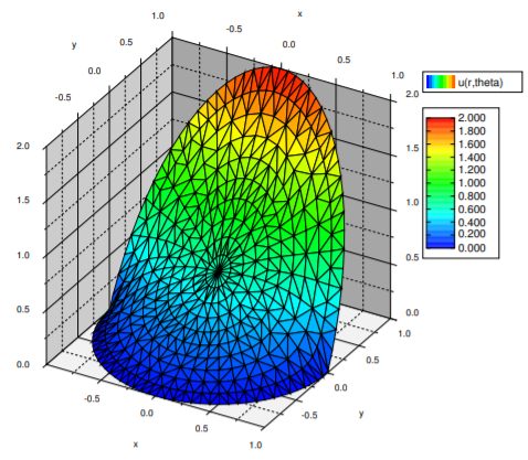
We now simply write the solution (see Figure $4$ ) by multiplying by $r^{n}$ in the right places.

$u (r, θ) = \frac{2}{π} + r \sin (θ) + \sum_{n = 1}^{\infty} \frac{- 4 r^{2 n}}{π (4 n^{2} - 1)} \cos (2 n θ) .$

Three-dimensional surface over the unit disc, height 0 to 2. Half the rim is held at 0 and lies low; over the other half the surface swells into a dome reaching 2 at the rim, with the centre only about 0.6 to 0.7. — Figure $4$ : The solution of the Dirichlet problem with boundary data $0$ for $y less than 0$ and $2 y$ for $y greater than 0$ .

Poisson Kernel

There is another way to solve the Dirichlet problem with the help of an integral kernel. That is, we will find a function $P (r, θ, α)$ called the Poisson kernelto the power 1 such that

$u (r, θ) = \frac{1}{2 π} \int_{- π}^{π} P (r, θ, α) g (α) d α .$

While the integral will generally not be solvable analytically, it can be evaluated numerically. In fact, unless the boundary data is given as a Fourier series already, it will be much easier to numerically evaluate this formula as there is only one integral to evaluate.

The formula also has theoretical applications. For instance, as $P (r, θ, α)$ will have infinitely many derivatives, then via differentiating under the integral we find that the solution $u (r, θ)$ has infinitely many derivatives, at least when inside the circle, $r less than 1$ . By infinitely many derivatives what you should think of is that $u (r, θ)$ has “no corners” and all of its partial derivatives exist too and also have “no corners”.

We will compute the formula for $P (r, θ, α)$ from the series solution, and this idea can be applied anytime you have a convenient series solution where the coefficients are obtained via integration. Hence you can apply this reasoning to obtain such integral kernels for other equations, such as the heat equation. The computation is long and tedious, but not overly difficult. Since the ideas are often applied in similar contexts, it is good to understand how this computation works.

What we do is start with the series solution and replace the coefficients with the integrals that compute them. Then we try to write everything as a single integral. We must use a different dummy variable for the integration and hence we use $α$ instead of $θ$ .

$\begin{matrix} u (r, θ) = \frac{a_{0}}{2} + \sum_{n = 1}^{\infty} a_{n} r^{n} \cos (n θ) + b_{n} r^{n} \sin (n θ) \\ = \underset{\frac{a_{0}}{2}}{\underset{⏟}{(\frac{1}{2 π} \int_{- π}^{π} g (α) d α)}} + \sum_{n = 1}^{\infty} \underset{a_{n}}{\underset{⏟}{(\frac{1}{π} \int_{- π}^{π} g (α) \cos (n α) d α)}} r^{n} \cos (n θ) \\ + \underset{b_{n}}{\underset{⏟}{(\frac{1}{π} \int_{- π}^{π} g (α) \sin (n α) d α)}} r^{n} \sin (n θ) \\ = \frac{1}{2 π} \int_{- π}^{π} (g (α) + 2 \sum_{n = 1}^{\infty} g (α) \cos (n α) r^{n} \cos (n θ) + g (α) \sin (n α) r^{n} \sin (n θ)) d α \\ = \frac{1}{2 π} \int_{- π}^{π} \underset{P (r, θ, α)}{\underset{⏟}{(1 + 2 \sum_{n = 1}^{\infty} r^{n} (\cos (n α) \cos (n θ) + \sin (n α) \sin (n θ)))}} g (α) d α \end{matrix}$

OK, so we have what we wanted, the expression in the parentheses is the Poisson kernel, $P (r, θ, α)$ . However, we can do a lot better. It is still given as a series, and we would really like to have a nice simple expression for it. We must work a little harder. The trick is to rewrite everything in terms of complex exponentials. Let us work just on the kernel.

$\begin{matrix} P (r, θ, α) = 1 + 2 \sum_{n = 1}^{\infty} r^{n} (\cos (n α) \cos (n θ) + \sin (n α) \sin (n θ)) \\ = 1 + 2 \sum_{n = 1}^{\infty} r^{n} \cos (n (θ - α)) \\ = 1 + 2 \sum_{n = 1}^{\infty} r^{n} (e^{i n (θ - α)} + e^{- i n (θ - α)}) \\ = 1 + \sum_{n = 1}^{\infty} (r e^{i (θ - α)})^{n} + \sum_{n = 1}^{\infty} (r e^{- i (θ - α)})^{n} . \end{matrix}$

In the above expression we recognize the geometric series. That is, recall from calculus that as long as $| z | less than 1$ , then

$\sum_{n = 1}^{\infty} z^{n} = \frac{z}{1 - z} .$

Note that $n$ starts at $1$ and that is why we have the $z$ in the numerator. It is the standard geometric series multiplied by $z$ . Let us continue with the computation.

$\begin{matrix} P (r, θ, α) = 1 + \sum_{n = 1}^{\infty} (r e^{i (θ - α)})^{n} + \sum_{n = 1}^{\infty} (r e^{- i (θ - α)})^{n} \\ = 1 + \frac{r e^{i (θ - α)}}{1 - r e^{i (θ - α)}} + \frac{r e^{- i (θ - α)}}{1 - r e^{- i (θ - α)}} \\ = \frac{(1 - r e^{i (θ - α)}) (1 - r e^{- i (θ - α)}) + (1 - r e^{- i (θ - α)}) r e^{i (θ - α)} + (1 - r e^{i (θ - α)}) r e^{- i (θ - α)}}{(1 - r e^{i (θ - α)}) (1 - r e^{- i (θ - α)})} \\ = \frac{1 - r^{2}}{1 - r e^{i (θ - α)} - r e^{- i (θ - α)} + r^{2}} \\ = \frac{1 - r^{2}}{1 - 2 r \cos (θ - α) + r^{2}} . \end{matrix}$

Now that’s a formula we can live with. The solution to the Dirichlet problem using the Poisson kernel is

$u (r, θ) = \frac{1}{2 π} \int_{- π}^{π} \frac{1 - r^{2}}{1 - 2 r \cos (θ - α) + r^{2}} g (α) d α .$

Sometimes the formula for the Poisson kernel is given together with the constant $\frac{1}{2 π}$ , in which case we should of course not leave it in front of the integral. Also, often the limits of the integral are given as $0$ to $2 π$ ; everything inside is $2 π$ -periodic in $α$ , so this does not change the integral.

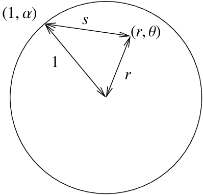
Let us not leave the Poisson kernel without explaining its geometric meaning. Let $s$ be the distance from $(r, θ)$ to $open parenthesis 1, α close parenthesis$ . You may recall from calculus that this distance $s$ in polar coordinates is given precisely by the square root of $1 - 2 r \cos (θ - α) + r^{2}$ . That is, the Poisson kernel is really the formula

$\frac{1 - r^{2}}{s^{2}} .$

Diagram of a circle with a radius labelled 1 drawn to a rim point (1, alpha), a segment labelled r from the centre to an interior point (r, theta), and a segment s joining those two points. — Figure $5$

One final note we make about the formula is to note that it is really a weighted average of the boundary values. First let us look at what happens at the origin, that is when $r equals 0$ .

$\begin{matrix} u (0, 0) = \frac{1}{2 π} \int_{- π}^{π} \frac{1 - 0^{2}}{1 - 2 (0) \cos (θ - α) + 0^{2}} g (α) d α \\ = \frac{1}{2 π} \int_{- π}^{π} g (α) d α . \end{matrix}$

So $u open parenthesis 0, 0 close parenthesis$ is precisely the average value of $g (θ)$ and therefore the average value of $u$ on the boundary. This is a general feature of harmonic functions, the value at some point $p$ is equal to the average of the values on a circle centered at $p$ .

What the formula says is that the value of the solution at any point in the circle is a weighted average of the boundary data $g (θ)$ . The kernel is bigger when $(r, θ)$ is closer to $open parenthesis 1, α close parenthesis$ . Therefore when computing $u (r, θ)$ we give more weight to the values $g (α)$ when $open parenthesis 1, α close parenthesis$ is closer to $(r, θ)$ and less weight to the values $g (θ)$ when $open parenthesis 1, α close parenthesis$ far from $(r, θ)$ .

Function graph showing y = (1-r^2)/(1-2*r*cos(x)+r^2) on x in [-3.14, 3.14] and y = 1 on x in [-3.14, 3.14]. Adjustable parameter: Radius r of the point in the disc (r) = 0.5. Viewing window: x from -3.8 to 3.8, y from -0.5 to 4.2. — The kernel P(r, θ, α) = (1 − r²)/(1 − 2r cos(θ − α) + r²) plotted against the boundary angle α, for an observation angle θ = 0: the horizontal axis says which boundary point, the vertical axis says how much weight it gets. Drag r out from the centre. At r = 0 the kernel lies flat on the dashed line at 1 — that is exactly the mean value property just proved, u(0, 0) = the average of g. By r = 0.6 it is a spike of height 4 over α = 0 while the far side of the circle has sunk to 0.25. The area underneath never changes, so this is re-weighting, not growth — which is also why a fast-wiggling boundary condition like cos(10θ) is felt at the boundary and dies before the middle of the disc.

Footnotes

[1] Named for the French mathematician Siméon Denis Poisson (1781 – 1840).

Adapted from Differential Equations for Engineers by Jiří Lebl (Oklahoma State University), hosted on LibreTexts (math.libretexts.org) and licensed under CC BY-SA 4.0. Changes were made. License: CC-BY-SA-4.0.