5.3 Linear Inequalities in One Variable with Applications

Learning Objectives

After completing this section, you should be able to:

1. Graph inequalities in one variable.
2. Solve linear inequalities in one variable.
3. Construct a linear inequality to solve applications.

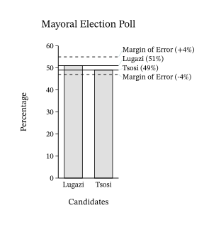
In this section, we will study linear inequalities in one variable. Inequalities can be used when the possible values (answers) in a certain situation are numerous, not just a few, or when the exact value (answer) is not known but it is known to be within a range of possible values. There are many real-world scenarios that can be represented by linear inequalities. For example, consider the survey of the mayoral election in Figure 5.5 Surveys and polls are usually conducted with only a small group of people. The margin of error indicates a range of how the actual group of voters would vote given the results of the survey. This range can be expressed using inequalities.

Another example involves college tuition. Say a local community college charges $113 per credit hour. You budget $1,500 for tuition this fall semester. What are the number of credit hours that you could take this fall? Since this answer could be many different values, it can be expressed as an inequality.

Graphing Inequalities on the Number Line

In Algebraic Expressions, we introduced equality and the $=$ symbol. In this section, we look at inequality and the symbols $<$, $>$, $\le$, and $\ge$. The table below summarizes the symbols and their meaning.

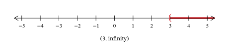
Suppose you had the inequality statement $x>3$. What possible number or numbers would make the inequality $x>3$ true? If you are thinking, "$x$ could be 4," that's correct, but $x$ could also be 5, 6, 37, 1 million, or even 3.001. The number of solutions is infinite; any number greater than 3 is a solution to the inequality $x>3$.

Rather than trying to list all possible solutions, we show all the solutions to the inequality $x>3$ on the number line. All the numbers to the right of 3 on the number line are shaded, to show that all numbers greater than 3 are solutions. At the number 3 itself, an open parenthesis is drawn, since the number 3 is not part of the solutions of $x>3$.

We can also represent inequalities using interval notation. There is no upper end to the solution to this inequality. In interval notation, we express $x>3$ as $\left(3,\infty \right)$. The symbol $\infty$ is read as "infinity." Infinity is not an actual number. Figure 5.6 shows both the number line and the interval notation for $x>3$.

We used the left parenthesis symbol to show that the endpoint of the inequality is not included. Parentheses are used when the endpoints are not included as a possible answer to the inequality. The notation for inequalities on a number line and in interval notation use the same symbols to express the endpoints of intervals.

The inequality $x\le 1$ means all numbers less than or equal to 1. To illustrate that solution on a number line, we first put a bracket at $x=1$; brackets are used when the endpoint is included. We then shade in all the numbers to the left of 1, to show that all numbers less than one are solutions. There is no lower end to those numbers. We write $x\le 1$ in interval notation as $\left(-\infty ,1\right]$. The symbol $-\infty$ is read as "negative infinity." Figure 5.7 shows both the number line and interval notation for $x=1$.

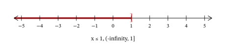
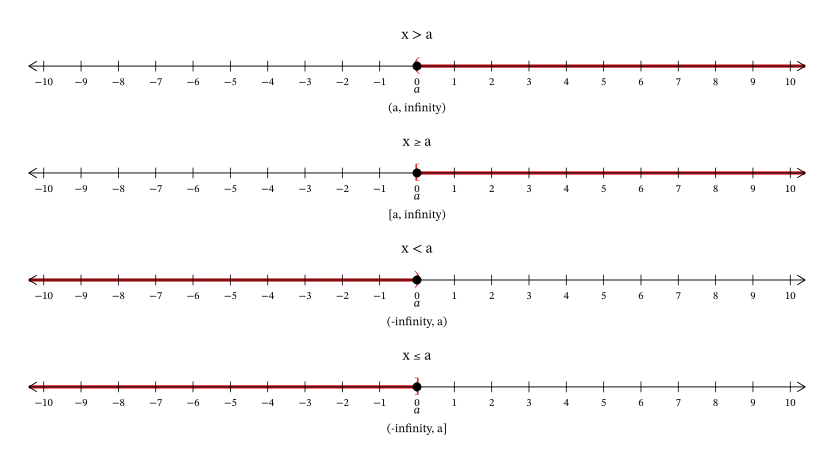
Figure 5.8 summarizes the general representations in both number line form and interval notation of solutions for $x>a$, $x<a$, $x\ge a$, and $x\le a$.

Solving Linear Inequalities

A linear inequality is much like a linear equation—but the equal sign is replaced with an inequality sign. A linear inequality is an inequality in one variable that can be written in one of the forms $$ax+b<c,ax+b\le c,ax+b\ge c,$$ or $ax+b>c,$ where $a$, $b$, and $c$ are all real numbers.

When we solved linear equations, we were able to use the properties of equality to add, subtract, multiply, or divide both sides and still keep the equality. Similar properties hold true for inequalities. We can add or subtract the same quantity from both sides of an inequality and still keep the inequality. For example, we know that 2 is less than 4, i.e., $2<4$. If we add 6 to both sides of this inequality, we still have a true statement:

$$\begin{array}{ccc}\hfill 2+6& \hfill <\hfill & 4+6\hfill \\ \hfill 8& \hfill <\hfill & 10\hfill \end{array}$$

The same would happen if we subtracted 6 from both sides of the inequality; the statement would stay true:

$$\begin{array}{ccc}\hfill 2-6& \hfill <\hfill & 4-6\hfill \\ \hfill -4& \hfill <\hfill & -2\hfill \end{array}$$

Notice that the inequality signs stayed the same. This leads us to the Addition and Subtraction Properties of Inequality.

We can add or subtract the same quantity from both sides of an inequality and still keep the inequality the same. But what happens to an inequality when we divide or multiply both sides by a number? Let's first multiply and divide both sides by a positive number, starting with an inequality we know is true, $10<15$. We will multiply and divide this inequality by 5:

$$\begin{array}{cccccc}\hfill 10& \hfill <\hfill & 15\hfill & \hfill 10& \hfill <\hfill & 15\hfill \\ \hfill 10\left(5\right)& \hfill ?\hfill & 15\left(5\right)\hfill & \hfill \frac{10}{5}& \hfill ?\hfill & \frac{15}{5}\hfill \\ \hfill 50& \hfill ?\hfill & 75\hfill & \hfill 2& \hfill ?\hfill & 3\hfill \\ \hfill 50& \hfill <\hfill & 75\left(\text{true}\right)\hfill & \hfill 2& \hfill <\hfill & 3\left(\text{true}\right)\hfill \end{array}$$

The inequality signs stayed the same. Does the inequality stay the same when we divide or multiply by a negative number? Let's use our inequality $10<15$ to find out, multiplying it and dividing it by $-5$:

$$\begin{array}{cccccc}\hfill 10& \hfill <\hfill & 15\hfill & \hfill 10& \hfill <\hfill & 15\hfill \\ \hfill 10\left(-5\right)& \hfill ?\hfill & 15\left(-5\right)\hfill & \hfill \frac{10}{-5}& \hfill ?\hfill & \frac{15}{-5}\hfill \\ \hfill -50& \hfill ?\hfill & -75\hfill & \hfill -2& \hfill ?\hfill & -3\hfill \\ \hfill -50& \hfill >\hfill & -75\left(\text{true}\right)\hfill & \hfill -2& \hfill >\hfill & -3\left(\text{true}\right)\hfill \end{array}$$

Notice that when we filled in the inequality signs, the inequality signs reversed their direction in order to make it true! To summarize, when we divide or multiply an inequality by a positive number, the inequality sign stays the same. When we divide or multiply an inequality by a negative number, the inequality sign reverses. This gives us the Multiplication and Division Property of Inequality.

To summarize, when we divide or multiply an inequality by:

• a positive number, the inequality sign stays the same.
• a negative number, the inequality sign reverses.

Solving Applications with Linear Inequalities

Many real-life situations require us to solve inequalities. The method we will use to solve applications with linear inequalities is very much like the one we used when we solved applications with equations. We will read the problem and make sure all the words are understood. Next, we will identify what we are looking for and assign a variable to represent it. We will restate the problem in one sentence to make it easy to translate into an inequality. Then, we will solve the inequality.

Sometimes an application requires the solution to be a whole number, but the algebraic solution to the inequality is not a whole number. In that case, we must round the algebraic solution to a whole number. The context of the application will determine whether we round up or down.

Key Terms

• linear inequality
• Addition and Subtraction Property of Linear Inequalities
• Multiplication and Division Property of Linear Inequalities

Key Concepts

• Inequalities can be used when the possible values (answers) in a certain situation are numerous, or when the exact value (answer) is not known, but it is known to be within a range of possible values.
• Linear inequalities can be represented using a number line or using interval notation.

Formulas

• For any numbers $a$, $b$, and $,$ if $a<b$, then $a+c<b+c$ and $a-c<b-c$.
• For any numbers $a$, $b$, and $c$, if $a>b$, then $a+c>b+c$ and $a-c>b-c$.
• For any numbers $a$, $b$, and $c$,
  multiply or divide by a positive:
  if $a<b$ and $c>0$, then $ac<bc$ and $\frac{a}{c}<\frac{b}{c}$
  if $a>b$ and $c>0$, then $ac>bc$ and $\frac{a}{c}>\frac{b}{c}$
  multiply or divide by a negative:
  if $a<b$ and $c<0$, then $ac>bc$ and $\frac{a}{c}>\frac{b}{c}$
  if $a>b$ and $c<0$, then $ac<bc$ and $\frac{a}{c}<\frac{b}{c}$