
10.5 Graphs of the Trigonometric Functions
In this section, we return to our discussion of the circular (trigonometric) functions as functions of real numbers and pick up where we left off in Sections 10.2.1 and 10.3.1. As usual, we begin our study with the functions and .
Graphs of the Cosine and Sine Functions
From Theorem 10.5 in Section 10.2.1, we know that the domain of and of is all real numbers, and the range of both functions is . The Even / Odd Identities in Theorem 10.12 tell us for all real numbers and for all real numbers . This means is an even function, while is an odd function.1 Another important property of these functions is that for coterminal angles and , and . Said differently, and for all real numbers and any integer . This last property is given a special name.
We have already seen a family of periodic functions in Section 2.1: the constant functions. However, despite being periodic a constant function has no period. (We'll leave that odd gem as an exercise for you.) Returning to the circular functions, we see that by Definition 10.3, is periodic, since for any integer . To determine the period of , we need to find the smallest real number so that for all real numbers or, said differently, the smallest positive real number such that for all real numbers . We know that for all real numbers but the question remains if any smaller real number will do the trick. Suppose and for all real numbers . Then, in particular, so that . From this we know is a multiple of and, since the smallest positive multiple of is itself, we have the result. Similarly, we can show is also periodic with as its period.2 Having period essentially means that we can completely understand everything about the functions and by studying one interval of length , say .3 In some advanced texts, the interval of choice is .
One last property of the functions and is worth pointing out: both of these functions are continuous and smooth. Recall from Section 3.1 that geometrically this means the graphs of the cosine and sine functions have no jumps, gaps, holes in the graph, asymptotes, corners or cusps. As we shall see, the graphs of both and meander nicely and don't cause any trouble. We summarize these facts in the following theorem.
In the chart above, we followed the convention established in Section 1.6 and used as the independent variable and as the dependent variable.4 This allows us to turn our attention to graphing the cosine and sine functions in the Cartesian Plane. To graph , we make a table as we did in Section 1.6 using some of the `common values' of in the interval . This generates a portion of the cosine graph, which we call the `fundamental cycle' of .
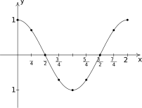
A few things about the graph above are worth mentioning. First, this graph represents only part of the graph of . To get the entire graph, we imagine `copying and pasting' this graph end to end infinitely in both directions (left and right) on the -axis. Secondly, the vertical scale here has been greatly exaggerated for clarity and aesthetics. Below is an accurate-to-scale graph of showing several cycles with the `fundamental cycle' plotted thicker than the others. The graph of is usually described as `wavelike' – indeed, many of the applications involving the cosine and sine functions feature modeling wavelike phenomena.

We can plot the fundamental cycle of the graph of similarly, with similar results.
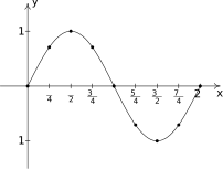
As with the graph of , we provide an accurately scaled graph of below with the fundamental cycle highlighted.

It is no accident that the graphs of and are so similar. Using a cofunction identity along with the even property of cosine, we have
Recalling Section 1.7, we see from this formula that the graph of is the result of shifting the graph of to the right units. A visual inspection confirms this.
Now that we know the basic shapes of the graphs of and , we can use Theorem 1.7 in Section 1.7 to graph more complicated curves. To do so, we need to keep track of the movement of some key points on the original graphs. We choose to track the values , , , and . These `quarter marks' correspond to quadrantal angles, and as such, mark the location of the zeros and the local extrema of these functions over exactly one period. Before we begin our next example, we need to review the concept of the `argument' of a function as first introduced in Section 1.4. For the function , the argument of is . We shall have occasion, however, to refer to the argument of the cosine, which in this case is . Loosely stated, the argument of a trigonometric function is the expression `inside' the function.
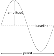
The functions in Example 10.5.1 are examples of sinusoids. Roughly speaking, a sinusoid is the result of taking the basic graph of or and performing any of the transformations5 mentioned in Section 1.7. Sinusoids can be characterized by four properties: period, amplitude, phase shift and vertical shift. We have already discussed period, that is, how long it takes for the sinusoid to complete one cycle. The standard period of both and is , but horizontal scalings will change the period of the resulting sinusoid. The amplitude of the sinusoid is a measure of how `tall' the wave is, as indicated in the figure below. The amplitude of the standard cosine and sine functions is , but vertical scalings can alter this.
The phase shift of the sinusoid is the horizontal shift experienced by the fundamental cycle. We have seen that a phase (horizontal) shift of to the right takes to since . As the reader can verify, a phase shift of to the left takes to . The vertical shift of a sinusoid is exactly the same as the vertical shifts in Section 1.7. In most contexts, the vertical shift of a sinusoid is assumed to be , but we state the more general case below. The following theorem, which is reminiscent of Theorem 1.7 in Section 1.7, shows how to find these four fundamental quantities from the formula of the given sinusoid.
We note that in some scientific and engineering circles, the quantity mentioned in Theorem 10.23 is called the phase of the sinusoid. Since our interest in this book is primarily with graphing sinusoids, we focus our attention on the horizontal shift induced by .
The proof of Theorem 10.23 is a direct application of Theorem 1.7 in Section 1.7 and is left to the reader. The parameter , which is stipulated to be positive, is called the (angular) frequency of the sinusoid and is the number of cycles the sinusoid completes over a interval. We can always ensure using the Even/Odd Identities.6 We now test out Theorem 10.23 using the functions and featured in Example 10.5.1. First, we write in the form prescribed in Theorem 10.23,
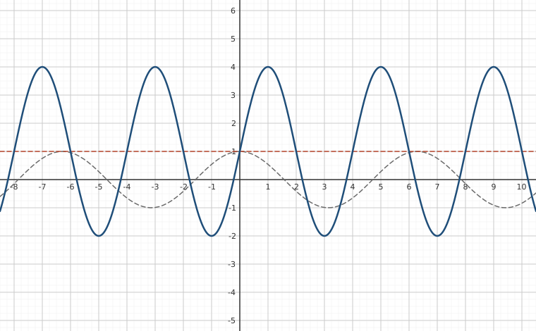
so that , , and . According to Theorem 10.23, the period of is , the amplitude is , the phase shift is (indicating a shift to the right unit) and the vertical shift is (indicating a shift up unit.) All of these match with our graph of . Moreover, if we start with the basic shape of the cosine graph, shift it unit to the right, unit up, stretch the amplitude to and shrink the period to , we will have reconstructed one period of the graph of . In other words, instead of tracking the five `quarter marks' through the transformations to plot , we can use five other pieces of information: the phase shift, vertical shift, amplitude, period and basic shape of the cosine curve. Turning our attention now to the function in Example 10.5.1, we first need to use the odd property of the sine function to write it in the form required by Theorem 10.23
We find , , and . The period is then , the amplitude is , the phase shift is (indicating a shift right units) and the vertical shift is up . Note that, in this case, all of the data match our graph of with the exception of the phase shift. Instead of the graph starting at , it ends there. Remember, however, that the graph presented in Example 10.5.1 is only one portion of the graph of . Indeed, another complete cycle begins at , and this is the cycle Theorem 10.23 is detecting. The reason for the discrepancy is that, in order to apply Theorem 10.23, we had to rewrite the formula for using the odd property of the sine function. Note that whether we graph using the `quarter marks' approach or using the Theorem 10.23, we get one complete cycle of the graph, which means we have completely determined the sinusoid.
Note that each of the answers given in Example 10.5.2 is one choice out of many possible answers. For example, when fitting a sine function to the data, we could have chosen to start at taking . In this case, the phase shift is so for an answer of . Alternatively, we could have extended the graph of to the left and considered a sine function starting at , and so on. Each of these formulas determine the same sinusoid curve and their formulas are all equivalent using identities. Speaking of identities, if we use the sum identity for cosine, we can expand the formula to yield
Similarly, using the sum identity for sine, we get
Making these observations allows us to recognize (and graph) functions as sinusoids which, at first glance, don't appear to fit the forms of either or .
It is important to note that in order for the technique presented in Example 10.5.3 to fit a function into one of the forms in Theorem 10.23, the arguments of the cosine and sine function much match. That is, while is a sinusoid, is not.9 It is also worth mentioning that, had we chosen instead of as we worked through Example 10.5.3, our final answers would have looked different. The reader is encouraged to rework Example 10.5.3 using to see what these differences are, and then for a challenging exercise, use identities to show that the formulas are all equivalent. The general equations to fit a function of the form into one of the forms in Theorem 10.23 are explored in Exercise.
Graphs of the Secant and Cosecant Functions
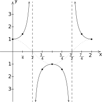
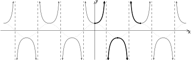
We now turn our attention to graphing . Since , we can use our table of values for the graph of and take reciprocals. We know from Section 10.3.1 that the domain of excludes all odd multiples of , and sure enough, we run into trouble at and since at these values. Using the notation introduced in Section 4.2, we have that as , , so . (See Section 10.3.1 for a more detailed analysis.) Similarly, we find that as , ; as , ; and as , . This means we have a pair of vertical asymptotes to the graph of , and . Since is periodic with period , it follows that is also.10 Below we graph a fundamental cycle of along with a more complete graph obtained by the usual `copying and pasting.'11
As one would expect, to graph we begin with and take reciprocals of the corresponding -values. Here, we encounter issues at , and . Proceeding with the usual analysis, we graph the fundamental cycle of below along with the dotted graph of for reference. Since and are merely phase shifts of each other, so too are and .
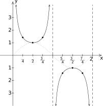
Once again, our domain and range work in Section 10.3.1 is verified geometrically in the graph of .
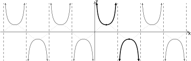
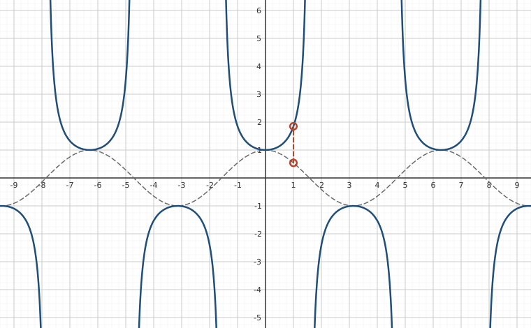
Note that, on the intervals between the vertical asymptotes, both and are continuous and smooth. In other words, they are continuous and smooth on their domains.12 The following theorem summarizes the properties of the secant and cosecant functions. Note that all of these properties are direct results of them being reciprocals of the cosine and sine functions, respectively.
In the next example, we discuss graphing more general secant and cosecant curves.
Before moving on, we note that it is possible to speak of the period, phase shift and vertical shift of secant and cosecant graphs and use even/odd identities to put them in a form similar to the sinusoid forms mentioned in Theorem 10.23. Since these quantities match those of the corresponding cosine and sine curves, we do not spell this out explicitly. Finally, since the ranges of secant and cosecant are unbounded, there is no amplitude associated with these curves.
Graphs of the Tangent and Cotangent Functions
Finally, we turn our attention to the graphs of the tangent and cotangent functions. When constructing a table of values for the tangent function, we see that is undefined at and , in accordance with our findings in Section 10.3.1. As , and , so that producing a vertical asymptote at . Using a similar analysis, we get that as , ; as , ; and as , . Plotting this information and performing the usual `copy and paste' produces:
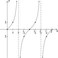
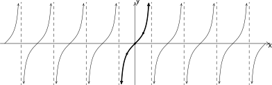
From the graph, it appears as if the tangent function is periodic with period . To prove that this is the case, we appeal to the sum formula for tangents. We have:
which tells us the period of is at most . To show that it is exactly , suppose is a positive real number so that for all real numbers . For , we have , which means is a multiple of . The smallest positive multiple of is itself, so we have established the result. We take as our fundamental cycle for the interval , and use as our `quarter marks' , , , and . From the graph, we see confirmation of our domain and range work in Section 10.3.1.
It should be no surprise that behaves similarly to . Plotting over the interval results in the graph below.
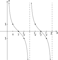
From these data, it clearly appears as if the period of is , and we leave it to the reader to prove this.13 We take as one fundamental cycle the interval with quarter marks: , , , and . A more complete graph of is below, along with the fundamental cycle highlighted as usual. Once again, we see the domain and range of as read from the graph matches with what we found analytically in Section 10.3.1.
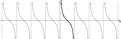
The properties of the tangent and cotangent functions are summarized below. As with Theorem 10.24, each of the results below can be traced back to properties of the cosine and sine functions and the definition of the tangent and cotangent functions as quotients thereof.
As with the secant and cosecant functions, it is possible to extend the notion of period, phase shift and vertical shift to the tangent and cotangent functions as we did for the cosine and sine functions in Theorem 10.23. Since the number of classical applications involving sinusoids far outnumber those involving tangent and cotangent functions, we omit this. The ambitious reader is invited to formulate such a theorem, however.
Exercises
In Exercises -, graph one cycle of the given function. State the period, amplitude, phase shift and vertical shift of the function.
In Exercises -, graph one cycle of the given function. State the period of the function.
In Exercises -, use Example 10.5.3 as a guide to show that the function is a sinusoid by rewriting it in the forms and for and .
- In Exercises -, you should have noticed a relationship between the phases for the and . Show that if , then where .
- Let be an angle measured in radians and let be a point on the terminal side of when it is drawn in standard position. Use Theorem 10.3 and the sum identity for sine in Theorem 10.15 to show that (with ) can be rewritten as .
- With the help of your classmates, express the domains of the functions in Examples 10.5.4 and 10.5.5 using extended interval notation. (We will revisit this in Section 10.7.)
In Exercises -, verify the identity by graphing the right and left hand sides on a calculator.
In Exercises -, graph the function with the help of your calculator and discuss the given questions with your classmates.
- . Is this function periodic? If so, what is the period?
- . What appears to be the horizontal asymptote of the graph?
- . Graph on the same set of axes and describe the behavior of .
- . What's happening as ?
- . Graph on the same set of axes and describe the behavior of .
- . Graph on the same set of axes and describe the behavior of .
- . Graph on the same set of axes and describe the behavior of .
- Show that a constant function is periodic by showing that for all real numbers . Then show that has no period by showing that you cannot find a smallest number such that for all real numbers . Said another way, show that for all real numbers for ALL values of , so no smallest value exists to satisfy the definition of `period'.
Answers
Period: Amplitude: Phase Shift: Vertical Shift:
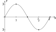
Figure 10.166 Period: Amplitude: Phase Shift: Vertical Shift:
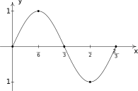
Figure 10.167 Period: Amplitude: Phase Shift: Vertical Shift:
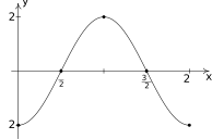
Figure 10.168 Period: Amplitude: Phase Shift: Vertical Shift:
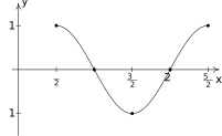
Figure 10.169 Period: Amplitude: Phase Shift: Vertical Shift:
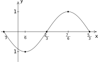
Figure 10.170 Period: Amplitude: Phase Shift: Vertical Shift:
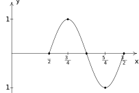
Figure 10.171 Period: Amplitude: Phase Shift: Vertical Shift:
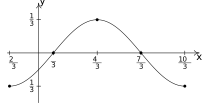
Figure 10.172 Period: Amplitude: Phase Shift: Vertical Shift: 4
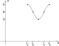
Figure 10.173 Period: Amplitude: Phase Shift: (You need to use to find this.)14 Vertical Shift:
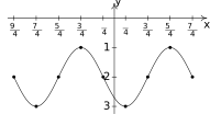
Figure 10.174 Period: Amplitude: Phase Shift: (You need to use to find this.)15 Vertical Shift:
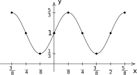
Figure 10.175 Period: Amplitude: Phase Shift: Vertical Shift:
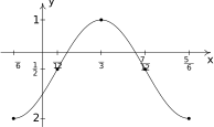
Figure 10.176 Period: Amplitude: Phase Shift: (You need to use to find this.)16 Vertical Shift:
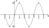
Figure 10.177 Period:
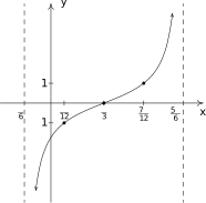
Figure 10.178 Period:
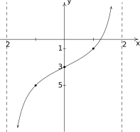
Figure 10.179 is equivalent to via the Even / Odd identity for tangent. Period:
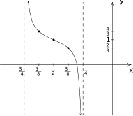
Figure 10.180 Start with Period:
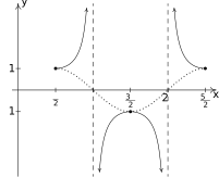
Figure 10.181 Start with Period:
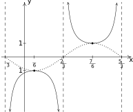
Figure 10.182 Start with Period:
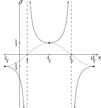
Figure 10.183 Start with Period:
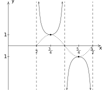
Figure 10.184 Start with Period:
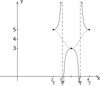
Figure 10.185 Start with Period:
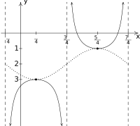
Figure 10.186 Period:
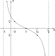
Figure 10.187 Period:
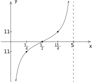
Figure 10.188 Period:
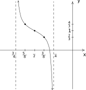
Figure 10.189
Adapted from Precalculus, 3rd corrected edition, by Carl Stitz and Jeff Zeager (stitz-zeager.com), licensed under CC BY-NC-SA 3.0. Changes were made: reformatted as an accessible XYZ web edition. License: CC-BY-NC-SA-3.0.