
10.1 Angles and their Measure
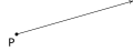
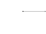
This section begins our study of Trigonometry and to get started, we recall some basic definitions from Geometry. A ray is usually described as a `half-line' and can be thought of as a line segment in which one of the two endpoints is pushed off infinitely distant from the other, as pictured below. The point from which the ray originates is called the initial point of the ray.
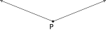
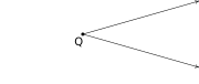
When two rays share a common initial point they form an angle and the common initial point is called the vertex of the angle. Two examples of what are commonly thought of as angles are
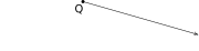
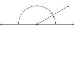
However, the two figures below also depict angles - albeit these are, in some sense, extreme cases. In the first case, the two rays are directly opposite each other forming what is known as a straight angle; in the second, the rays are identical so the `angle' is indistinguishable from the ray itself.

The measure of an angle is a number which indicates the amount of rotation that separates the rays of the angle. There is one immediate problem with this, as pictured below.
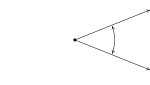
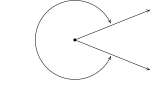
Which amount of rotation are we attempting to quantify? What we have just discovered is that we have at least two angles described by this diagram.1 Clearly these two angles have different measures because one appears to represent a larger rotation than the other, so we must label them differently. In this book, we use lower case Greek letters such as (alpha), (beta), (gamma) and (theta) to label angles. So, for instance, we have
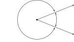
One commonly used system to measure angles is degree measure. Quantities measured in degrees are denoted by the familiar `' symbol. One complete revolution as shown below is , and parts of a revolution are measured proportionately.2 Thus half of a revolution (a straight angle) measures , a quarter of a revolution (a right angle) measures and so on.
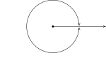
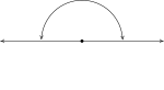
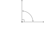
Note that in the above figure, we have used the small square `' to denote a right angle, as is commonplace in Geometry. Recall that if an angle measures strictly between and it is called an acute angle and if it measures strictly between and it is called an obtuse angle. It is important to note that, theoretically, we can know the measure of any angle as long as we know the proportion it represents of entire revolution.3 For instance, the measure of an angle which represents a rotation of of a revolution would measure , the measure of an angle which constitutes only of a revolution measures and an angle which indicates no rotation at all is measured as .
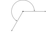
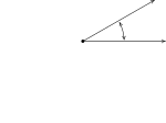
Using our definition of degree measure, we have that represents the measure of an angle which constitutes of a revolution. Even though it may be hard to draw, it is nonetheless not difficult to imagine an angle with measure smaller than . There are two ways to subdivide degrees. The first, and most familiar, is decimal degrees. For example, an angle with a measure of would represent a rotation halfway between and , or equivalently, of a full rotation. This can be taken to the limit using Calculus so that measures like make sense.4 The second way to divide degrees is the Degree - Minute - Second (DMS) system. In this system, one degree is divided equally into sixty minutes, and in turn, each minute is divided equally into sixty seconds.5 In symbols, we write and , from which it follows that . To convert a measure of to the DMS system, we start by noting that . Converting the partial amount of degrees to minutes, we find . Converting the partial amount of minutes to seconds gives . Putting it all together yields
On the other hand, to convert to decimal degrees, we first compute and . Then we find
Recall that two acute angles are called complementary angles if their measures add to . Two angles, either a pair of right angles or one acute angle and one obtuse angle, are called supplementary angles if their measures add to . In the diagram below, the angles and are supplementary angles while the pair and are complementary angles.
In practice, the distinction between the angle itself and its measure is blurred so that the sentence ` is an angle measuring ' is often abbreviated as `.' It is now time for an example.
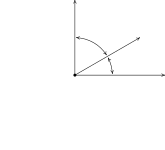
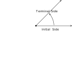
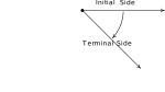
Up to this point, we have discussed only angles which measure between and , inclusive. Ultimately, we want to use the arsenal of Algebra which we have stockpiled in Chapters 1 through 9 to not only solve geometric problems involving angles, but also to extend their applicability to other real-world phenomena. A first step in this direction is to extend our notion of `angle' from merely measuring an extent of rotation to quantities which can be associated with real numbers. To that end, we introduce the concept of an oriented angle. As its name suggests, in an oriented angle, the direction of the rotation is important. We imagine the angle being swept out starting from an initial side and ending at a terminal side, as shown below. When the rotation is counter-clockwise9 from initial side to terminal side, we say that the angle is positive; when the rotation is clockwise, we say that the angle is negative.
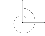
At this point, we also extend our allowable rotations to include angles which encompass more than one revolution. For example, to sketch an angle with measure we start with an initial side, rotate counter-clockwise one complete revolution (to take care of the `first' ) then continue with an additional counter-clockwise rotation, as seen below.
To further connect angles with the Algebra which has come before, we shall often overlay an angle diagram on the coordinate plane. An angle is said to be in standard position if its vertex is the origin and its initial side coincides with the positive -axis. Angles in standard position are classified according to where their terminal side lies. For instance, an angle in standard position whose terminal side lies in Quadrant I is called a `Quadrant I angle'. If the terminal side of an angle lies on one of the coordinate axes, it is called a quadrantal angle. Two angles in standard position are called coterminal if they share the same terminal side.10 In the figure below, and are two coterminal Quadrant II angles drawn in standard position. Note that , or equivalently, . We leave it as an exercise to the reader to verify that coterminal angles always differ by a multiple of .11 More precisely, if and are coterminal angles, then where is an integer.12
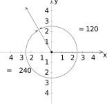
Two coterminal angles, and , in standard position.
Note that since there are infinitely many integers, any given angle has infinitely many coterminal angles, and the reader is encouraged to plot the few sets of coterminal angles found in Example 10.1.2 to see this. We are now just one step away from completely marrying angles with the real numbers and the rest of Algebra. To that end, we recall this definition from Geometry.
While Definition 10.1 is quite possibly the `standard' definition of , the authors would be remiss if we didn't mention that buried in this definition is actually a theorem. As the reader is probably aware, the number is a mathematical constant - that is, it doesn't matter which circle is selected, the ratio of its circumference to its diameter will have the same value as any other circle. While this is indeed true, it is far from obvious and leads to a counterintuitive scenario which is explored in the Exercises. Since the diameter of a circle is twice its radius, we can quickly rearrange the equation in Definition 10.1 to get a formula more useful for our purposes, namely:
This tells us that for any circle, the ratio of its circumference to its radius is also always constant; in this case the constant is . Suppose now we take a portion of the circle, so instead of comparing the entire circumference to the radius, we compare some arc measuring units in length to the radius, as depicted below. Let be the central angle subtended by this arc, that is, an angle whose vertex is the center of the circle and whose determining rays pass through the endpoints of the arc. Using proportionality arguments, it stands to reason that the ratio should also be a constant among all circles, and it is this ratio which defines the radian measure of an angle.
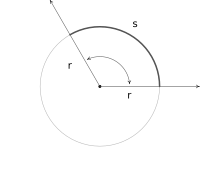
The radian measure of is .
To get a better feel for radian measure, we note that an angle with radian measure means the corresponding arc length equals the radius of the circle , hence . When the radian measure is , we have ; when the radian measure is , , and so forth. Thus the radian measure of an angle tells us how many `radius lengths' we need to sweep out along the circle to subtend the angle .
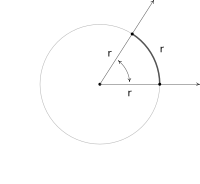
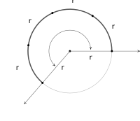
has radian measure
has radian measure
Since one revolution sweeps out the entire circumference , one revolution has radian measure . From this we can find the radian measure of other central angles using proportions, just like we did with degrees. For instance, half of a revolution has radian measure , a quarter revolution has radian measure , and so forth. Note that, by definition, the radian measure of an angle is a length divided by another length so that these measurements are actually dimensionless and are considered `pure' numbers. For this reason, we do not use any symbols to denote radian measure, but we use the word `radians' to denote these dimensionless units as needed. For instance, we say one revolution measures ` radians,' half of a revolution measures ` radians,' and so forth.
As with degree measure, the distinction between the angle itself and its measure is often blurred in practice, so when we write `', we mean is an angle which measures radians.13 We extend radian measure to oriented angles, just as we did with degrees beforehand, so that a positive measure indicates counter-clockwise rotation and a negative measure indicates clockwise rotation.14 Much like before, two positive angles and are supplementary if and complementary if . Finally, we leave it to the reader to show that when using radian measure, two angles and are coterminal if and only if for some integer .
It is worth mentioning that we could have plotted the angles in Example 10.1.3 by first converting them to degree measure and following the procedure set forth in Example 10.1.2. While converting back and forth from degrees and radians is certainly a good skill to have, it is best that you learn to `think in radians' as well as you can `think in degrees'. The authors would, however, be derelict in our duties if we ignored the basic conversion between these systems altogether. Since one revolution counter-clockwise measures and the same angle measures radians, we can use the proportion , or its reduced equivalent, , as the conversion factor between the two systems. For example, to convert to radians we find , or simply . To convert from radian measure back to degrees, we multiply by the ratio . For example, is equal to .15 Of particular interest is the fact that an angle which measures in radian measure is equal to .
We summarize these conversions below.
In light of Example 10.1.3 and Equation 10.1, the reader may well wonder what the allure of radian measure is. The numbers involved are, admittedly, much more complicated than degree measure. The answer lies in how easily angles in radian measure can be identified with real numbers. Consider the Unit Circle, , as drawn below, the angle in standard position and the corresponding arc measuring units in length. By definition, and the fact that the Unit Circle has radius 1, the radian measure of is so that, once again blurring the distinction between an angle and its measure, we have . In order to identify real numbers with oriented angles, we make good use of this fact by essentially `wrapping' the real number line around the Unit Circle and associating to each real number an oriented arc on the Unit Circle with initial point .
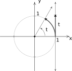
Viewing the vertical line as another real number line demarcated like the -axis, given a real number , we `wrap' the (vertical) interval around the Unit Circle in a counter-clockwise fashion. The resulting arc has a length of units and therefore the corresponding angle has radian measure equal to . If , we wrap the interval clockwise around the Unit Circle. Since we have defined clockwise rotation as having negative radian measure, the angle determined by this arc has radian measure equal to . If , we are at the point on the -axis which corresponds to an angle with radian measure . In this way, we identify each real number with the corresponding angle with radian measure .
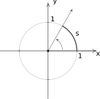
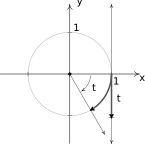
On the Unit Circle, .
Identifying with an angle.
Identifying with an angle.
Applications of Radian Measure: Circular Motion
Now that we have paired angles with real numbers via radian measure, a whole world of applications awaits us. Our first excursion into this realm comes by way of circular motion. Suppose an object is moving as pictured below along a circular path of radius from the point to the point in an amount of time .
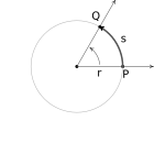
Here represents a displacement so that means the object is traveling in a counter-clockwise direction and indicates movement in a clockwise direction. Note that with this convention the formula we used to define radian measure, namely , still holds since a negative value of incurred from a clockwise displacement matches the negative we assign to for a clockwise rotation. In Physics, the average velocity of the object, denoted and read as `-bar', is defined as the average rate of change of the position of the object with respect to time.16 As a result, we have . The quantity has units of and conveys two ideas: the direction in which the object is moving and how fast the position of the object is changing. The contribution of direction in the quantity is either to make it positive (in the case of counter-clockwise motion) or negative (in the case of clockwise motion), so that the quantity quantifies how fast the object is moving - it is the speed of the object. Measuring in radians we have thus and
The quantity is called the average angular velocity of the object. It is denoted by and is read `omega-bar'. The quantity is the average rate of change of the angle with respect to time and thus has units . If is constant throughout the duration of the motion, then it can be shown17 that the average velocities involved, namely and , are the same as their instantaneous counterparts, and , respectively. In this case, is simply called the `velocity' of the object and is the instantaneous rate of change of the position of the object with respect to time.18 Similarly, is called the `angular velocity' and is the instantaneous rate of change of the angle with respect to time.
If the path of the object were `uncurled' from a circle to form a line segment, then the velocity of the object on that line segment would be the same as the velocity on the circle. For this reason, the quantity is often called the linear velocity of the object in order to distinguish it from the angular velocity, . Putting together the ideas of the previous paragraph, we get the following.
We need to talk about units here. The units of are , the units of are length only, and the units of are . Thus the left hand side of the equation has units , whereas the right hand side has units . The supposed contradiction in units is resolved by remembering that radians are a dimensionless quantity and angles in radian measure are identified with real numbers so that the units reduce to the units . We are long overdue for an example.
It is worth noting that the quantity in Example 10.1.5 is called the ordinary frequency of the motion and is usually denoted by the variable . The ordinary frequency is a measure of how often an object makes a complete cycle of the motion. The fact that suggests that is also a frequency. Indeed, it is called the angular frequency of the motion. On a related note, the quantity is called the period of the motion and is the amount of time it takes for the object to complete one cycle of the motion. In the scenario of Example 10.1.5, the period of the motion is 24 hours, or one day.
The concepts of frequency and period help frame the equation in a new light. That is, if is fixed, points which are farther from the center of rotation need to travel faster to maintain the same angular frequency since they have farther to travel to make one revolution in one period's time. The distance of the object to the center of rotation is the radius of the circle, , and is the `magnification factor' which relates and . We will have more to say about frequencies and periods in Section 11.1. While we have exhaustively discussed velocities associated with circular motion, we have yet to discuss a more natural question: if an object is moving on a circular path of radius with a fixed angular velocity (frequency) , what is the position of the object at time ? The answer to this question is the very heart of Trigonometry and is answered in the next section.
Exercises
In Exercises -, convert the angles into the DMS system. Round each of your answers to the nearest second.
In Exercises -, convert the angles into decimal degrees. Round each of your answers to three decimal places.
In Exercises -, graph the oriented angle in standard position. Classify each angle according to where its terminal side lies and then give two coterminal angles, one of which is positive and the other negative.
In Exercises -, convert the angle from degree measure into radian measure, giving the exact value in terms of .
In Exercises -, convert the angle from radian measure into degree measure.
In Exercises -, sketch the oriented arc on the Unit Circle which corresponds to the given real number.
- A yo-yo which is 2.25 inches in diameter spins at a rate of 4500 revolutions per minute. How fast is the edge of the yo-yo spinning in miles per hour? Round your answer to two decimal places.
- How many revolutions per minute would the yo-yo in exercise have to complete if the edge of the yo-yo is to be spinning at a rate of 42 miles per hour? Round your answer to two decimal places.
- In the yo-yo trick `Around the World,' the performer throws the yo-yo so it sweeps out a vertical circle whose radius is the yo-yo string. If the yo-yo string is 28 inches long and the yo-yo takes 3 seconds to complete one revolution of the circle, compute the speed of the yo-yo in miles per hour. Round your answer to two decimal places.
- A computer hard drive contains a circular disk with diameter 2.5 inches and spins at a rate of 7200 RPM (revolutions per minute). Find the linear speed of a point on the edge of the disk in miles per hour.
- A rock got stuck in the tread of my tire and when I was driving 70 miles per hour, the rock came loose and hit the inside of the wheel well of the car. How fast, in miles per hour, was the rock traveling when it came out of the tread? (The tire has a diameter of 23 inches.)
- The Giant Wheel at Cedar Point is a circle with diameter 128 feet which sits on an 8 foot tall platform making its overall height is 136 feet. (Remember this from Exercise in Section 7.2?) It completes two revolutions in 2 minutes and 7 seconds.20 Assuming the riders are at the edge of the circle, how fast are they traveling in miles per hour?
Consider the circle of radius pictured below with central angle , measured in radians, and subtended arc of length . Prove that the area of the shaded sector is .
(Hint: Use the proportion .)
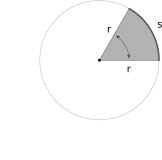
Figure 10.42
In Exercises -, use the result of Exercise to compute the areas of the circular sectors with the given central angles and radii.
- Imagine a rope tied around the Earth at the equator. Show that you need to add only feet of length to the rope in order to lift it one foot above the ground around the entire equator. (You do NOT need to know the radius of the Earth to show this.)
- With the help of your classmates, look for a proof that is indeed a constant.
Answers
is a Quadrant IV angle coterminal with and
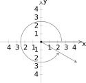
Figure 10.43 is a Quadrant III angle coterminal with and
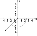
Figure 10.44 is a Quadrant II angle coterminal with and
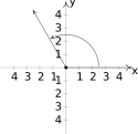
Figure 10.45 is a Quadrant I angle coterminal with and
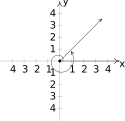
Figure 10.46 lies on the positive -axis coterminal with and
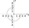
Figure 10.47 is a Quadrant II angle coterminal with and
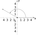
Figure 10.48 is a Quadrant I angle coterminal with and
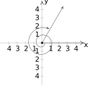
Figure 10.49 is a Quadrant III angle coterminal with and
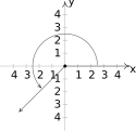
Figure 10.50 is a Quadrant II angle coterminal with and
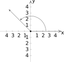
Figure 10.51 is a Quadrant IV angle coterminal with and
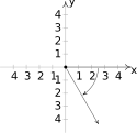
Figure 10.52 lies on the negative -axis coterminal with and
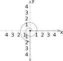
Figure 10.53 is a Quadrant I angle coterminal with and
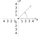
Figure 10.54 lies on the negative -axis coterminal with and
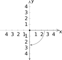
Figure 10.55 is a Quadrant III angle coterminal with and
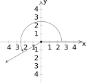
Figure 10.56 is a Quadrant I angle coterminal with and
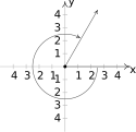
Figure 10.57 lies on the negative -axis coterminal with and
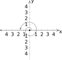
Figure 10.58 lies on the positive -axis coterminal with and
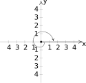
Figure 10.59 is a Quadrant IV angle coterminal with and
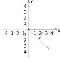
Figure 10.60 is a Quadrant IV angle coterminal with and
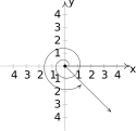
Figure 10.61 is a Quadrant IV angle coterminal with and
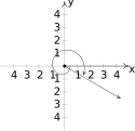
Figure 10.62 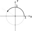
Figure 10.63 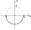
Figure 10.64 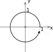
Figure 10.65 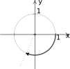
Figure 10.66 (between 1 and 2 revolutions)
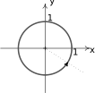
Figure 10.67 - About 30.12 miles per hour
- About 6274.52 revolutions per minute
- About 3.33 miles per hour
- About 53.55 miles per hour
- 70 miles per hour
- About 4.32 miles per hour
- square units
- square units
- square units
- square units
- square units
- square units
Adapted from Precalculus, 3rd corrected edition, by Carl Stitz and Jeff Zeager (stitz-zeager.com), licensed under CC BY-NC-SA 3.0. Changes were made: reformatted as an accessible XYZ web edition. License: CC-BY-NC-SA-3.0.