8.3 Hypothesis Test for One Mean

There are three methods used to test hypotheses:

The Traditional Method (Critical Value Method)

There are five steps in hypothesis testing when using the traditional method:

Identify the claim and formulate the hypotheses.
Compute the test statistic.
Compute the critical value(s) and state the rejection rule (the rule by which you will reject the null hypothesis (H₀).
Make the decision to reject or not reject the null hypothesis by comparing the test statistic to the critical value(s). Reject H₀ when the test statistic is in the critical tail(s).
Summarize the results and address the claim using context and units from the research question.

Steps ii and iii do not have to be in that order so make sure you know the difference between the critical value, which comes from the stated significance level $α$ , and the test statistic, which is calculated from the sample data.

Note: The test statistic and the critical value(s) come from the same distribution and will usually have the same letter such as z, t, or F. The critical value(s) will have a subscript with the lower tail area $open parenthesis z sub α, z sub 1 – α, z sub α / 2 close parenthesis$ or an asterisk next to it (z*) to distinguish it from the test statistic.

You can find the critical value(s) or test statistic in any order, but make sure you know the difference when you compare the two. The critical value is found from α and is the start of the shaded area called the critical region (also called rejection region or area). The test statistic is computed using sample data and may or may not be in the critical region.

The critical value(s) is set before you begin (a priori) by the level of significance you are using for your test. This critical value(s) defines the shaded area known as the rejection area. The test statistic for this example is the z-score we find using the sample data that is then compared to the shaded tail(s). When the test statistic is in the shaded rejection area, you reject the null hypothesis. When your test statistic is not in the shaded rejection area, then you fail to reject the null hypothesis. Depending on if your claim is in the null or the alternative, the sample data may or may not support your claim.

The P-value Method

Most modern statistics and research methods utilize this method with the advent of computers and graphing calculators.

There are five steps in hypothesis testing when using the p-value method:

Identify the claim and formulate the hypotheses.
Compute the test statistic.
Compute the p-value.
Make the decision to reject or not reject the null hypothesis by comparing the p-value with $α$ . Reject H0 when the p-value ≤ $α$ .
Summarize the results and address the claim.

The ideas below review the process of evaluating hypothesis tests with p-values:

The null hypothesis represents a skeptic’s position or a position of no difference. We reject this position only if the evidence strongly favors the alternative hypothesis.
A small p-value means that if the null hypothesis is true, there is a low probability of seeing a point estimate at least as extreme as the one we saw. We interpret this as strong evidence in favor of the alternative hypothesis.
The p-value is constructed in such a way that we can directly compare it to the significance level ( $α$ ) to determine whether to reject H₀. We reject the null hypothesis if the p-value is smaller than the significance level, $α$ , which is usually 0.05. Otherwise, we fail to reject H₀.
We should always state the conclusion of the hypothesis test in plain language use context and units so non-statisticians can also understand the results.

The Confidence Interval Method (results are in the same units as the data)

There are four steps in hypothesis testing when using the confidence interval method:

Identify the claim and formulate the hypotheses.
Compute confidence interval.
Make the decision to reject or not reject the null hypothesis by comparing the p-value with $α$ . Reject H₀ when the hypothesized value found in H₀ is outside the bounds of the confidence interval. We only will be doing a two-tailed version of this.
Summarize the results and address the claim.

For all 3 methods, Step i is the most important step. If you do not correctly set up your hypotheses then the next steps will be incorrect.

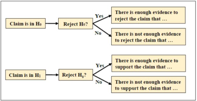
The decision and summary would be the same no matter which method you use. Figure 8-12 is a flow chart that may help with starting your summaries, but make sure you finish the sentence with context and units from the question.

Flow chart for writing test summaries. When the claim is in H0, reject H0? yes leads to there is enough evidence to reject the claim that…, and no leads to there is not enough evidence to reject the claim that…. When the claim is in H1, reject H0? yes leads to there is enough evidence to support the claim that…, and no leads to there is not enough evidence to support the claim that….

Figure 8-12

The hypothesis-testing framework is a very general tool, and we often use it without a second thought. If a person makes a somewhat unbelievable claim, we are initially skeptical. However, if there is sufficient evidence that supports the claim, we set aside our skepticism and reject the null hypothesis in favor of the alternative.

8.3.1 Z-Test

When the population standard deviation is known and stated in the problem, we will use the z-test.

Example 1

M&Ms candies advertise a mean weight of 0.8535 grams. A sample of 50 M&M candies are randomly selected from a bag of M&Ms and the mean is found to be $\bar{x}$ = 0.8472 grams. The standard deviation of the weights of all M&Ms is (somehow) known to be σ = 0.06 grams. A skeptic M&M consumer claims that the mean weight is less than what is advertised. Test this claim using the traditional method of hypothesis testing. Use a 5% level of significance.

Show solution

By letting $α$ = 0.05, we are allowing a 5% chance that the null hypothesis (average weight that is at least 0.8535 grams) is rejected when in actuality it is true.

1. Identify the Claim: The claim is “M&Ms candies have a mean weight that is less than 0.8535 grams.” This translates mathematically to µ < 0.8535 grams. Therefore, the null and alternative hypotheses are:

H0: µ = 0.8535

H1: µ < 0.8535 (claim)

This is a left-tailed test since the alternative hypothesis has a “less than” sign.

We are performing a test about a population mean. We can use the z-test because we were given a population standard deviation σ (not a sample standard deviation s). In practice, σ is rarely known and usually comes from a similar study or previous year’s data.

2. Find the Critical Value: The critical value for a left-tailed test with a level of significance $α$ = 0.05 is found in a way similar to finding the critical values from confidence intervals. Because we are using the z-test, we must find the critical value $z_{α}$ from the z (standard normal) distribution.

This is a left-tailed test since the sign in the alternative hypothesis is < (most of the time a left-tailed test will have a negative z-score test statistic).

Figure 8-13

First draw your curve and shade the appropriate tail with the area $α$ = 0.05. Usually the technology you are using only asks for the area in the left tail, which in this case is $α$ = 0.05. For the TI calculators, under the DISTR menu use invNorm(0.05,0,1) = –1.645. See Figure 8-13.

For Excel use =NORM.S.INV(0.05).

3. Find the Test Statistic: The formula for the test statistic is the z-score that we used back in the Central Limit Theorem section $z = \frac{\bar{x} - μ_{0}}{(\frac{σ}{\sqrt{n}})} = \frac{0.8472 - 0.8535}{(\frac{0.06}{\sqrt{50}})} = - 0.7425$ .

4. Make the Decision: Figure 8-14 shows both the critical value and the test statistic. There are only two possible correct answers for the decision step.

i. Reject H₀

ii. Fail to reject H₀

Figure 8-14

To make the decision whether to “Do not reject H₀” or “Reject H₀” using the traditional method, we must compare the test statistic z = –0.7425 with the critical value z_α = –1.645.

When the test statistic is in the shaded tail, called the rejection area, then we would reject H₀, if not then we fail to reject H₀. Since the test statistic z ≈ –0.7425 is in the unshaded region, the decision is: Do not reject H₀.

5. Summarize the Results: At 5% level of significance, there is not enough evidence to support the claim that the mean weight is less than 0.8535 grams.

Example 8-5 used the traditional critical value method. With the onset of computers, this method is outdated and the p-value and confidence interval methods are becoming more popular.

Most statistical software packages will give a p-value and confidence interval but not the critical value.

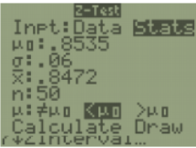
TI-84: Press the [STAT] key, go to the [TESTS] menu, arrow down to the [Z-Test] option and press the [ENTER] key. Arrow over to the [Stats] menu and press the [ENTER] key. Then type in value for the hypothesized mean (µ₀), standard deviation, sample mean, sample size, arrow over to the $\neq$ , <, > sign that is in the alternative hypothesis statement then press the [ENTER] key, arrow down to [Calculate] and press the [ENTER] key. Alternatively (If you have raw data in a list) Select the [Data] menu and press the [ENTER] key. Then type in the value for the hypothesized mean (µ₀), type in your list name (TI-84 L₁ is above the 1 key).

TI-84 Z-Test input screen with Stats selected: μ0 = .8535, σ = .06, x̄ = .8472, n = 50, alternative hypothesis μ < μ0 highlighted, with Calculate and Draw options below.

Press the [STAT] key, go to the [TESTS] menu, arrow down to either the [Z-Test] option and press the [ENTER] key. Arrow over to the [Stats] menu and press the [ENTER] key. Then type in value for the hypothesized mean (µ₀), standard deviation, sample mean, sample size, arrow over to the $\neq$ , <, > sign that is in the alternative hypothesis statement then press the [ENTER] key, arrow down to [Calculate] and press the [ENTER] key. Alternatively (If you have raw data in a list) Select the [Data] menu and press the [ENTER] key. Then type in the value for the hypothesized mean (µ₀), type in your list name (TI-84 L₁ is above the 1 key).

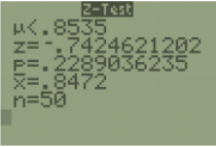
TI-84 Z-Test results screen: μ < .8535, z = −.7424621202, p = .2289036235, x̄ = .8472, n = 50.

The calculator returns the alternative hypothesis (check and make sure you selected the correct sign), the test statistic, p-value, sample mean, and sample size.

TI-89: Go in to the Stat/List Editor App. Select [F6] Tests. Select the first option Z-Test. Select Data if you have raw data in a list, select Stats if you have the summarized statistics given to you in the problem. If you have data, press [2nd] Var-Link, the go down to list1 in the main folder to select the list name. If you have statistics then enter the values. Leave Freq:1 alone, arrow over to the $\neq$ , <, > sign that is in the alternative hypothesis statement then press the [ENTER]key, arrow down to [Calculate] and press the [ENTER] key. The calculator returns the test statistic and the p-value.

Four TI-89 screens for a z-test: the Tests menu with 1:Z-Test highlighted, a Choose Input Method dialog with Stats selected, the Z Test input dialog with μ0 = .8535, σ = .06, x̄ = .8472, n = 50 and alternate hypothesis choices μ ≠ μ0, μ < μ0, μ > μ0, and the results screen showing μ < μ0, z = −.742462, P Value = .228904, x̄ = .8472, n = 50, σ = .06.

What is the p-value?

The p-value is the probability of observing an effect as least as extreme as in your sample data, assuming that the null hypothesis is true. The p-value is calculated based on the assumptions that the null hypothesis is true for the population and that the difference in the sample is caused entirely by random chance.

Recall the example at the beginning of the chapter.

Example 2

Suppose a manufacturer of a new laptop battery claims the mean life of the battery is 900 days with a standard deviation of 40 days. You are the buyer of this battery and you think this claim is inflated. You would like to test your belief because without a good reason you cannot get out of your contract. You take a random sample of 35 batteries and find that the mean battery life is 890 days. Test the claim using the p-value method. Let $α$ = 0.05.

Show solution

We had the following hypotheses:

H₀: μ = 900, since the manufacturer says the mean life of a battery is 900 days.

H₁: μ < 900, since you believe the mean life of the battery is less than 900 days.

The test statistic was found to be: $Z = \frac{\bar{x} - μ_{0}}{(\frac{σ}{\sqrt{n}})} = \frac{890 - 900}{(\frac{40}{\sqrt{35}})} = - 1.479$ .

The p-value is P( $\bar{x}$ < 890 | H₀ is true) = P( $\bar{x}$ < 890 | μ = 900) = P(Z < –1.479).

On the TI Calculator use normalcdf(-1E99,890,900,40/ $the square root of 35$ ) $\approx$ 0.0696. See Figure 8-15.

Figure 8-15

Alternatively, in Excel use =NORM.DIST(890,900,40/SQRT(35),TRUE) $\approx$ 0.0696.

The TI calculators will easily find the p-value for you.

Now compare the p-value = 0.0696 to $α$ = 0.05. Make the decision to reject or not reject the null hypothesis by comparing the p-value with $α$ . Reject H₀ when the p-value ≤ α, and do not reject H0 when the p-value > $α$ . The p-value for this example is larger than alpha 0.0696 > 0.05, therefore the decision is to not reject H₀.

Since we fail to reject the null, there is not enough evidence to indicate that the mean life of the battery is less than 900 days.

8.3.2 T-Test

When the population standard deviation is unknown, we will use the t-test.

Z Versus T

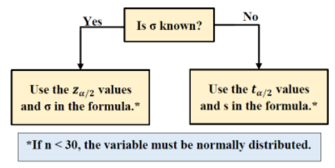
The z and t-tests are easy to mix up. Sometimes a standard deviation will be stated in the problem without specifying if it is a population’s standard deviation σ or the sample standard deviation s. If the standard deviation is in the same sentence that describes the sample or only raw data is given then this would be s. When you only have sample data, use the t-test.

Figure 8-16 is a flow chart to remind you when to use z versus t.

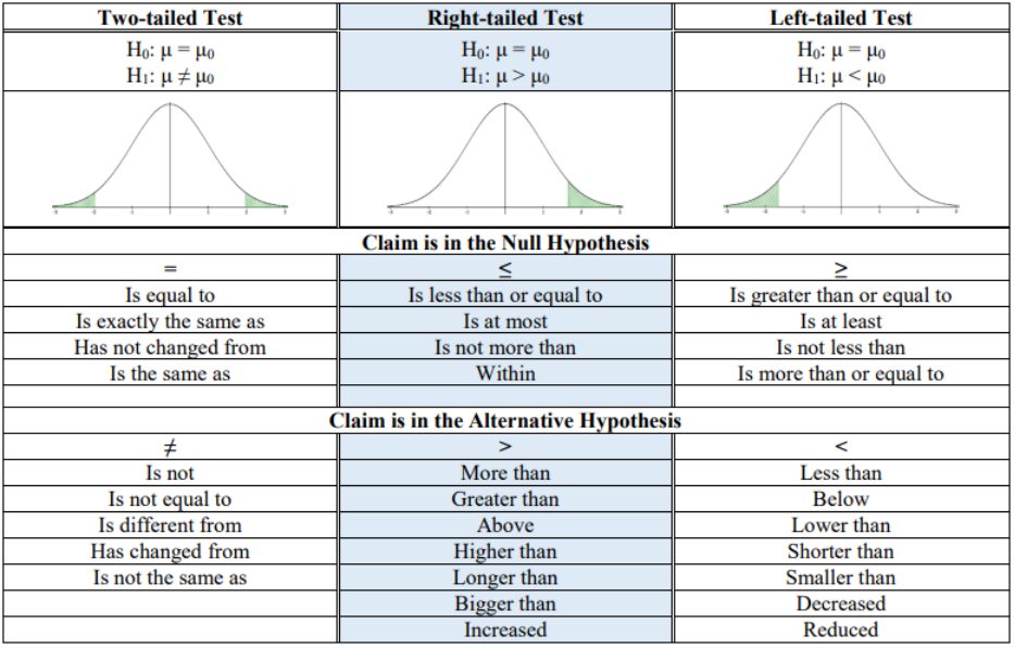
Flow chart asking is σ known? Yes leads to use the z sub α/2 values and σ in the formula; no leads to use the t sub α/2 values and s in the formula. A footnote reads: if n < 30, the variable must be normally distributed.

Figure 8-16

Use Figure 8-17 as a guide in setting up your hypotheses. The two-tailed test will always have a not equal ≠ sign in H₁ and both tails shaded. The right-tailed test will always have the greater than > sign in H₁ and the right tail shaded. The left-tailed test will always have a less than < sign in H₁ and the left tail shaded.

Hypothesis testing table with three columns: two-tailed test (H0: μ = μ0, H1: μ ≠ μ0, normal curve with both tails shaded), right-tailed test (H1: μ > μ0, right tail shaded), and left-tailed test (H1: μ < μ0, left tail shaded). Below, phrases when the claim is in the null hypothesis: = (is equal to, is exactly the same as, has not changed from), ≤ (is less than or equal to, is at most, is not more than, within), ≥ (is greater than or equal to, is at least, is not less than); and when the claim is in the alternative hypothesis: ≠ (is not, is not equal to, is different from, has changed from), > (more than, greater than, above, higher than, longer than, bigger than, increased), < (less than, below, lower than, shorter than, smaller than, decreased, reduced).

Figure 8-17

Example 3

The label on a particular brand of cream of mushroom soup states that (on average) there is 870 mg of sodium per serving. A nutritionist would like to test if the average is actually more than the stated value. To test this, 13 servings of this soup were randomly selected and amount of sodium measured. The sample mean was found to be 882.4 mg and the sample standard deviation was 24.3 mg. Assume that the amount of sodium per serving is normally distributed. Test this claim using the traditional method of hypothesis testing. Use the $α$ = 0.05 level of significance.

Solution

Step 1: State the hypotheses and identify the claim: The statement “the average is more (>) than 870” must be in the alternative hypothesis. Therefore, the null and alternative hypotheses are:

H₀: µ = 870

H₁: µ > 870 (claim)

This is a right-tailed test with the claim in the alternative hypothesis.

Step 2: Compute the test statistic: We are using the t-test because we are performing a test about a population mean. We must use the t-test (instead of the z-test) because the population standard deviation σ is unknown. (Note: be sure that you know why we are using the t-test instead of the z-test in general.)

The formula for the test statistic is $t = \frac{\bar{x} - μ_{0}}{(\frac{S}{\sqrt{n}})} = \frac{882.4 - 870}{(\frac{24.3}{\sqrt{13}})} = 1.8399$ .

Note: If you were given raw data use 1-var Stats on your calculator to find the sample mean, sample size and sample standard deviation.

Step 3: Compute the critical value(s): The critical value for a right-tailed test with a level of significance $α$ = 0.05 is found in a way similar to finding the critical values from confidence intervals.

Since we are using the t-test, we must find the critical value t_{1– $α$} from a t-distribution with the degrees of freedom, df = n – 1 = 13 –1 = 12. Use the DISTR menu invT option. Note that if you have an older TI-84 or a TI-83 calculator you need to have the invT program installed or use Excel.

Draw and label the t-distribution curve with the critical value as in Figure 8-18.

Figure 8-18

The critical value is t_{1– $α$} = 1.782 and the rejection rule becomes: Reject H₀ if the test statistic t ≥ t_{1– $α$} = 1.782.

Step 4: State the decision. Decision: Since the test statistic t =1.8399 is in the critical region, we should Reject H₀.

Step 5: State the summary. Summary: At the 5% significance level, we have sufficient evidence to say that the average amount of sodium per serving of cream of mushroom soup exceeds the stated 870 mg amount.

Example 8-7 Continued:

Use the prior example, but this time use the p-value method. Again, let the significance level be $α$ = 0.05.

Solution

Step 1: The hypotheses remain the same. H₀: µ = 870

H₁: µ > 870 (claim)

Step 2: The test statistic remains the same, $t = \frac{\bar{x} - μ_{0}}{(\frac{S}{\sqrt{n}})} = \frac{882.4 - 870}{(\frac{24.3}{\sqrt{13}})} = 1.8399$ .

Step 3: Compute the p-value.

For a right-tailed test, the p-value is found by finding the area to the right of the test statistic t = 1.8339 under a t-distribution with 12 degrees of freedom. See Figure 8-19.

Figure 8-19

Note that exact p-values for a t-test can only be found using a computer or calculator. For the TI calculators this is in the DISTR menu. Use tcdf(lower,upper,df).

For this example, we would have p-value = tcdf(1.8399,∞,12) = 0.0453.

Step 4: State the decision. The rejection rule: reject the null hypothesis if the p-value ≤ $α$ . Decision: Since the p-value = 0.0453 is less than $α$ = 0.05, we Reject H₀. This agrees with the decision from the traditional method. (These two methods should always agree!)

Step 5: State the summary. The summary remains the same as in the previous method. At the 5% significance level, we have sufficient evidence to say that the average amount of sodium per serving of cream of mushroom soup exceeds the stated 870 mg amount.

We can use technology to get the test statistic and p-value.

TI-84: If you have raw data, enter the data into a list before you go to the test menu. Press the [STAT] key, arrow over to the [TESTS] menu, arrow down to the [2:T-Test] option and press the [ENTER] key. Arrow over to the [Stats] menu and press the [ENTER] key. Then type in the hypothesized mean (µ₀), sample or population standard deviation, sample mean, sample size, arrow over to the $\neq$ , <, > sign that is the same as the problem’s alternative hypothesis statement then press the [ENTER] key, arrow down to [Calculate] and press the [ENTER] key. The calculator returns the t-test statistic and p-value.

Alternatively (If you have raw data in list one) Arrow over to the [Data] menu and press the [ENTER] key. Then type in the hypothesized mean (µ₀), L₁, leave Freq:1 alone, arrow over to the $\neq$ , <, > sign that is the same in the problem’s alternative hypothesis statement then press the [ENTER] key, arrow down to [Calculate] and press the [ENTER] key. The calculator returns the t-test statistic and the p-value.

TI-89: Go to the [Apps] Stat/List Editor, then press [2^nd] then F6 [Tests], then select 2: T-Test. Choose the input method, data is when you have entered data into a list previously or stats when you are given the mean and standard deviation already. Then type in the hypothesized mean (μ₀), sample standard deviation, sample mean, sample size (or list name (list1), and Freq: 1), arrow over to the $\neq$ , <, > and select the sign that is the same as the problem’s alternative hypothesis statement then press the [ENTER] key to calculate. The calculator returns the t-test statistic and p-value.

Example 4

The weight of the world’s smallest mammal is the bumblebee bat (also known as Kitti’s hog-nosed bat or Craseonycteris thonglongyai) is approximately normally distributed with a mean 1.9 grams. Such bats are roughly the size of a large bumblebee. A chiropterologist believes that the Kitti’s hog-nosed bats in a new geographical region under study has a different average weight than 1.9 grams. A sample of 10 bats weighed in grams in the new region are shown below. Use the confidence interval method to test the claim that mean weight for all bumblebee bats is not 1.9 g using a 10% level of significance.

Solution

Step 1: State the hypotheses and identify the claim. The key phrase is “mean weight not equal to 1.9 g.” In mathematical notation, this is μ ≠ 1.9. The not equal ≠ symbol is only allowed in the alternative hypothesis so the hypotheses would be:

H₀: μ = 1.9

H₁: μ ≠ 1.9

Step 2: Compute the confidence interval. First, find the t critical value using df = n – 1 = 9 and 90% confidence. In Excel t_$α$_/2 = T.INV(.1/2,9) = 1.833113.

Then use technology to find the sample mean and sample standard deviation and substitute in your numbers to the formula.

$\begin{aligned}
&\bar{x} \pm t_{\alpha / 2}\left(\frac{s}{\sqrt{n}}\right) \\
&\Rightarrow 1.985 \pm 1.833113\left(\frac{0.235242}{\sqrt{10}}\right) \\
&\Rightarrow 1.985 \pm 1.833113(0.07439) \\
&\Rightarrow 1.985 \pm 0.136365 \\
&\Rightarrow(1.8486,2.1214)
\end{aligned}$

The answer can be given as an inequality 1.8486 < µ < 2.1214

or in interval notation (1.8486, 2.1214).

Step 3: Make the decision: The rejection rule is to reject H0 when the hypothesized value found in H₀ is outside the bounds of the confidence interval. The null hypothesis was μ = 1.9 g. Since 1.9 is between the lower and upper boundary of the confidence interval 1.8486 < µ < 2.1214 then we would not reject H₀.

# Why the interval method and the test always agree - simulate the bat study
# 10,000 times with H0 TRUE (mu = 1.9, s ~ 0.235242, n = 10).
set.seed(9)
mu0 <- 1.9; sigma <- 0.235242; n <- 10
inside <- replicate(10000, {
  x  <- rnorm(n, mu0, sigma)
  ci <- mean(x) + c(-1, 1) * qt(0.95, n - 1) * sd(x) / sqrt(n)  # 90% t-interval
  mu0 > ci[1] && mu0 < ci[2]
})
mean(inside)    # ~0.90 of the intervals capture 1.9 -> fail to reject
mean(!inside)   # ~0.10 miss it -> exactly the alpha = 0.10 rejection rate

The sampling distribution, assuming the null hypothesis is true, will have a mean of μ = 1.9 and a standard error of $\frac{0.2352}{\sqrt{10}} = 0.07439$ . When we calculated the confidence interval using the sample mean of 1.985 the confidence interval captured the hypothesized mean of 1.9. See Figure 8-20.

Figure 8-20

Step 4: State the summary: At the 10% significance level, there is not enough evidence to support the claim that the population mean weight for bumblebee bats in the new geographical region is different from 1.9 g.

This interval can also be computed using a TI calculator or Excel.

TI-84: Enter the data in a list, choose Tests > TInterval. Select and highlight Data, change the list and confidence level to match the question. Choose Calculate.

Excel: Select Data Analysis > Descriptive Statistics: Note, you will need to change the cell reference numbers to where you copy and paste your data, only check the label box if you selected the label in the input range, and change the confidence level to 1 – $α$ .

Below is the Excel output. Excel only calculates the descriptive statistics with the margin of error.

Use Excel to find each piece of the interval $\bar{x} \pm t_{α / 2} (\frac{s}{\sqrt{n}})$ .

Excel $t sub α / 2$ = T.INV(0.1/2,9) = 1.8311.

$\begin{aligned}
&\bar{x} \pm t_{\alpha / 2}\left(\frac{s}{\sqrt{n}}\right) \\
&\Rightarrow 1.985 \pm 1.8311\left(\frac{0.2352}{\sqrt{10}}\right) \\
&\Rightarrow 1.985 \pm 1.8311(0.07439)
\end{aligned}$

Can you find the mean and standard error $\frac{s}{\sqrt{n}} = 0.07439$ in the Excel output?

$⇒ 1.985 ± 0.136365$

Can you find the margin of error $t_{\frac{α}{2}} (\frac{s}{\sqrt{n}}) = 0.136365$ in the Excel output?

Subtract and add the margin of error from the sample mean to get each confidence interval boundary (1.8486, 2.1214).

If we have raw data, Excel will do both the traditional and p-value method.

Example 8-8 Continued:

Use the prior example, but this time use the p-value method. Again, let the significance level be $α$ = 0.05.

Solution

Step 1: State the hypotheses. The hypotheses are: H₀: μ = 1.9

H₁: μ ≠ 1.9

Step 2: Compute the test statistic, $t = \frac{\bar{x} - μ_{0}}{(\frac{s}{\sqrt{n}})} = \frac{1.985 - 1.9}{(\frac{.235242}{\sqrt{10}})} = 1.1426$

Verify using Excel. Excel does not have a one-sample t-test, but it does have a two-sample t-test that can be used with a dummy column of zeros as the second sample to get the results for just one sample. Copy over the data into cell A1. In column B, next to the data, type in a dummy column of zeros, and label it Dummy. (We frequently use placeholders in statistics called dummy variables.)

Select the Data Analysis tool and then select t-Test: Paired Two Sample for Means, then select OK.

For the Variable 1 Range select the data in cells A1:A11, including the label. For the Variable 2 Range select the dummy column of zeros in cells B1:B11, including the label. Change the hypothesized mean to 1.9. Check the Labels box and change the alpha value to 0.10, then select OK.

Excel provides the following output:

Step 3: Compute the p-value. Since the alternative hypothesis has a ≠ symbol, use the Excel output next two-tailed p-value = 0.2826.

Step 4: Make the decision. For the p-value method we would compare the two-tailed p-value = 0.2826 to $α$ = 0.10. The rule is to reject H₀ if the p-value ≤ $α$ . In this case the p-value > $α$ , therefore we do not reject H₀. Again, the same decision as the confidence interval method.

For the critical value method, we would compare the test statistic t = 1.142625 with the critical values for a two-tailed test $t_{\frac{α}{2}}$ = ±1.833113. Since the test statistic is between –1.8331 and 1.8331 we would not reject H₀, which is the same decision using the p-value method or the confidence interval method.

Step 5: State the summary. There is not enough evidence to support the claim that the population mean weight for all bumblebee bats is not equal to 1.9 g.

One-Tailed Versus Two-Tailed Tests

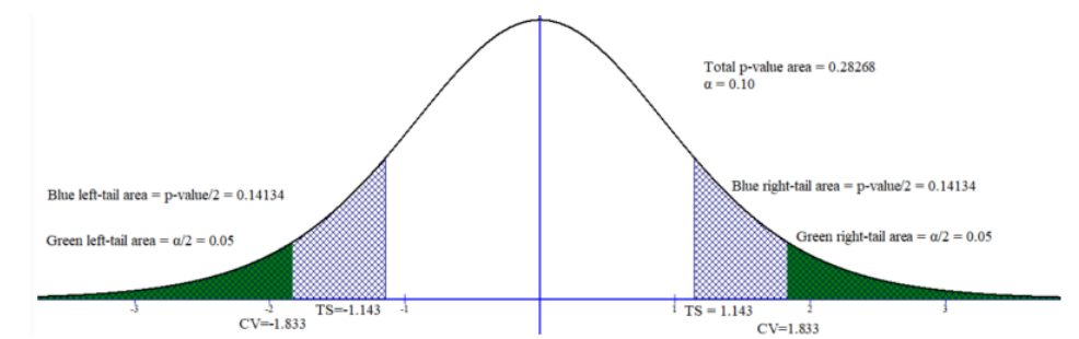
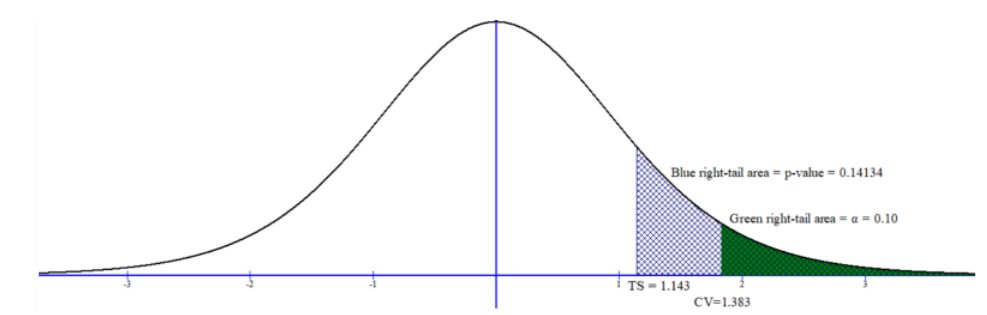
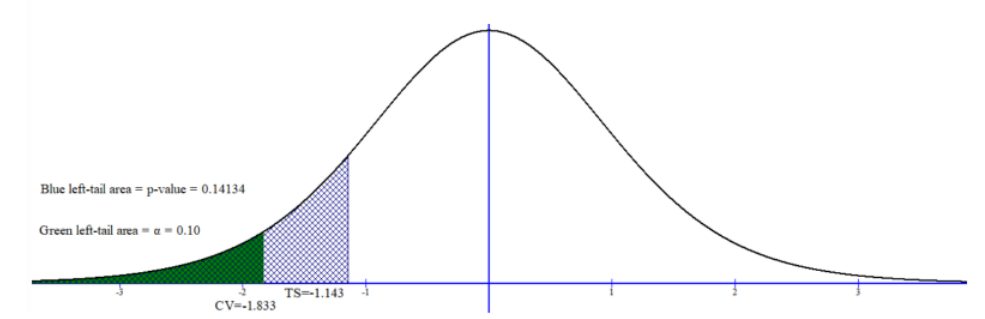
Most software packages do not ask which tailed test you are performing. Make sure you look at the sign in the alternative hypothesis to and determine which p-value to use. The difference is just what part of the picture you are looking at. In Excel, the critical value shown is for a one-tail test and does not specify left or right tail. The critical value in the output will always be positive, it is up to you to know if the critical value should be a negative or positive value. For example, Figures 8-21, 8-22, and 8-23 uses df = 9, $α$ = 0.10 to show all three tests comparing either the test statistic with the critical value or the p-value with $α$ .

Two-Tailed Test

The test statistic can be negative or positive depending on what side of the distribution it falls; however, the p-value is a probability and will always be a positive number between 0 and 1. See Figure 8-21.

Figure 8-21

Right-Tailed Test

If we happened to do a right-tailed test with df = 9 and $α$ = 0.10, the critical value t_{1- $α$} = 1.383 will be in the right tail and usually the test statistic will be a positive number. See Figure 8-22.

Figure 8-22

Left-Tailed Test

If we happened to do a left-tailed test with df = 9 and $α$ = 0.10, the critical value t_$α$ = –1.383 will be in the left tail and usually the test statistic will be a negative number. See Figure 8-23.

Figure 8-23

Adapted from Mostly Harmless Statistics by Rachel Webb (Portland State University), hosted on LibreTexts (stats.libretexts.org) and licensed under CC BY-SA 4.0. Changes were made. License: CC-BY-SA-4.0.