8.2 Type I and II Errors

How do you quantify really small? Is 5% or 10% or 15% really small? How do you decide? That depends on your field of study and the importance of the situation. Is this a pilot study? Is someone’s life at risk? Would you lose your job? Most industry standards use 5% as the cutoff point for how small is small enough, but 1%, 5% and 10% are frequently used depending on what the situation calls for.

Now, how small is small enough? To answer that, you really want to know the types of errors you can make in hypothesis testing.

The first error is if you say that H₀ is false, when in fact it is true. This means you reject H₀ when H₀ was true. The second error is if you say that H₀ is true, when in fact it is false. This means you fail to reject H₀ when H₀ is false.

Figure 8-4 shows that if we “Reject H₀ ” when H₀ is actually true, we are committing a type I error. The probability of committing a type I error is the Greek letter $α$ , pronounced alpha. This can be controlled by the researcher by choosing a specific level of significance $α$ .

Two-by-two decision table: reject H0 when H0 is true is a type I error; reject H0 when H0 is false is a correct decision; do not reject H0 when H0 is true is a correct decision; do not reject H0 when H0 is false is a type II error.

Figure 8-4

Figure 8-4 shows that if we “Do Not Reject H₀” when H₀ is actually false, we are committing a type II error. The probability of committing a type II error is denoted with the Greek letter β, pronounced beta. When we increase the sample size this will reduce β. The power of a test is 1 – β.

Example 1

A jury trial is about to take place to decide if a person is guilty of committing murder. The hypotheses for this situation would be:

$H sub 0$ : The defendant is innocent
$H sub 1$ : The defendant is not innocent

The jury has two possible decisions to make, either acquit or convict the person on trial, based on the evidence that is presented. There are two possible ways that the jury could make a mistake. They could convict an innocent person or they could let a guilty person go free. Both are bad news, but if the death penalty was sentenced to the convicted person, the justice system could be killing an innocent person. If a murderer is let go without enough evidence to convict them then they could possibly murder again. In statistics we call these two types of mistakes a type I and II error.

Figure 8-5 is a diagram to see the four possible jury decisions and two errors.

Figure 8-5

Definition

Type I Error is rejecting H₀ when H₀ is true, and Type II Error is failing to reject H₀ when H₀ is false.

# alpha is not just a threshold - it IS the long-run type I error rate.
# Simulate the battery test 10,000 times with H0 TRUE (mu really is 900).
set.seed(8)
mu0 <- 900; sigma <- 40; n <- 35
z <- replicate(10000, (mean(rnorm(n, mu0, sigma)) - mu0) / (sigma / sqrt(n)))
mean(z <= qnorm(0.05))   # left-tailed test at alpha = 0.05 -> rejects ~0.05
mean(z <= qnorm(0.01))   # tighten alpha to 0.01 -> rejects ~0.01
# Every one of those rejections is a type I error: H0 was true the whole time.

Since these are the only two possible errors, one can define the probabilities attached to each error.

$α$ = P(Type I Error) = P(Rejecting H₀ | H₀ is true)

β = P(Type II Error) = P(Failing to reject H₀ | H₀ is false)

Example 2

An investment company wants to build a new food cart. They know from experience that food carts are successful if they have on average more than 100 people a day walk by the location. They have a potential site to build on, but before they begin, they want to see if they have enough foot traffic. They observe how many people walk by the site every day over a month. They will build if there is more than an average of 100 people who walk by the site each day. In simple terms, explain what the type I & II errors would be using context from the problem.

Show solution

The hypotheses are: H₀: μ = 100 and H₁: μ > 100.

Sometimes it is helpful to use words next to your hypotheses instead of the formal symbols

H₀: μ ≤ 100 (Do not build)
H₁: μ > 100 (Build).

A type I error would be to reject the null when in fact it is true. Take your finger and cover up the null hypothesis (our decision is to reject the null), then what is showing? The alternative hypothesis is what action we take.

If we reject H₀ then we would build the new food cart. However, H₀ was actually true, which means that the mean was less than or equal to 100 people walking by.

In more simple terms, this would mean that our evidence showed that we have enough foot traffic to support the food cart. Once we build, though, there was not on average more than 100 people that walk by and the food cart may fail.

A type II error would be to fail to reject the null when in fact the null is false. Evidence shows that we should not build on the site, but this actually would have been a prime location to build on.

The missed opportunity of a type II error is not as bad as possibly losing thousands of dollars on a bad investment.

What is more severe of an error is dependent on what side of the desk you are sitting on. For instance, if a hypothesis is about miles per gallon for a new car the hypotheses may be set up differently depending on if you are buying the car or selling the car. For this course, the claim will be stated in the problem and always set up the hypotheses to match the stated claim. In general, the research question should be set up as some type of change in the alternative hypothesis.

Controlling for Type I Error

The significance level used by the researcher should be picked prior to collection and analyzing data. This is called “a priori,” versus picking α after you have done your analysis which is called “post hoc.” When deciding on what significance level to pick, one needs to look at the severity of the consequences of the type I and type II errors. For example, if the type I error may cause the loss of life or large amounts of money the researcher would want to set $α$ low.

Controlling for Type II Error

The power of a test is the complement of a type II error or correctly rejecting a false null hypothesis. You can increase the power of the test and hence decrease the type II error by increasing the sample size. Similar to confidence intervals, where we can reduce our margin of error when we increase the sample size. In general, we would like to have a high confidence level and a high power for our hypothesis tests. When you increase your confidence level, then in turn the power of the test will decrease. Calculating the probability of a type II error is a little more difficult and it is a conditional probability based on the researcher’s hypotheses and is not discussed in this course.

“‘That's right!’ shouted Vroomfondel, ‘we demand rigidly defined areas of doubt and uncertainty!’”

(Adams, 2002)

Visualizing $α$ and β

If $α$ increases that means the chances of making a type I error will increase. It is more likely that a type I error will occur. It makes sense that you are less likely to make type II errors, only because you will be rejecting H₀ more often. You will be failing to reject H₀less, and therefore, the chance of making a type II error will decrease. Thus, as α increases, β will decrease, and vice versa. That makes them seem like complements, but they are not complements. Consider one more factor – sample size.

Consider if you have a larger sample that is representative of the population, then it makes sense that you have more accuracy than with a smaller sample. Think of it this way, which would you trust more, a sample mean of 890 if you had a sample size of 35 or sample size of 350 (assuming a representative sample)? Of course, the 350 because there are more data points and so more accuracy. If you are more accurate, then there is less chance that you will make any error.

By increasing the sample size of a representative sample, you decrease β.

When the sample size becomes large, point estimates become more precise and any real differences in the mean and null value become easier to detect and recognize. Even a very small difference would likely be detected if we took a large enough sample size. Sometimes researchers will take such a large sample size that even the slightest difference is detected. While we still say that difference is statistically significant, it might not be practically significant. Statistically significant differences are sometimes so minor that they are not practically relevant. This is especially important to research: if we conduct a study, we want to focus on finding a meaningful result. We do not want to spend lots of money finding results that hold no practical value.

The role of a statistician in conducting a study often includes planning the size of the study. The statistician might first consult experts or scientific literature to learn what would be the smallest meaningful difference from the null value. They also would obtain some reasonable estimate for the standard deviation. With these important pieces of information, they would choose a sufficiently large sample size so that the power for the meaningful difference is perhaps 80% or 90%. While larger sample sizes may still be used, the statistician might advise against using them in some cases, especially in sensitive areas of research.

If we look at the following two sampling distributions in Figure 8-6, the one on the left represents the sampling distribution for the true unknown mean. The curve on the right represents the sampling distribution based on the hypotheses the researcher is making. Do you remember the difference between a sampling distribution, the distribution of a sample, and the distribution of the population? Revisit the Central Limit Theorem in Chapter 6 if needed.

If we start with $α$ = 0.05, the critical value is represented by the vertical green line at $z_{α}$ = 1.96. Then the blue shaded area to the right of this line represents $α$ . The area under the curve to the left of $z sub α / 2$ = 1.96 based on the researcher’s claim would represent β.

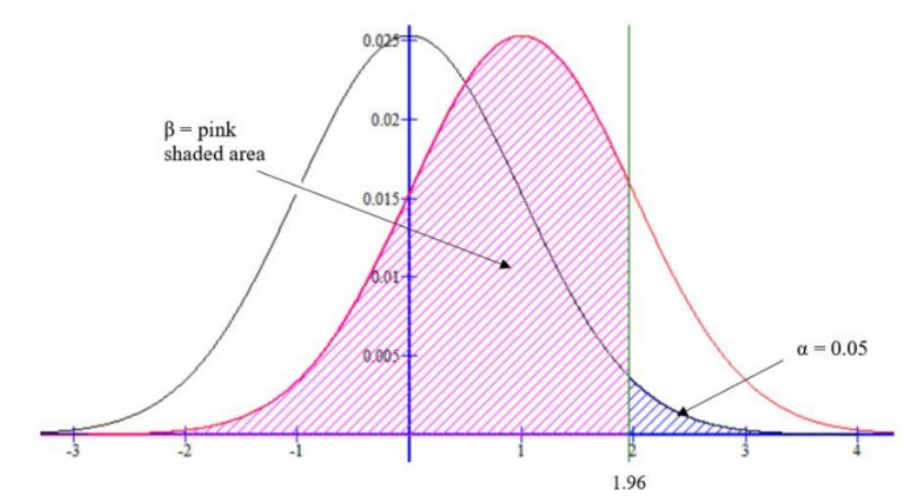
Two overlapping normal curves, a black curve centered at 0 and a red curve centered at 1, over an axis from −3 to 4. A green vertical line at 1.96 marks the critical value; the small blue hatched area under the black curve to its right is labeled α = 0.05, and the large pink hatched area under the red curve to its left is labeled β = pink shaded area.

Figure 8-6

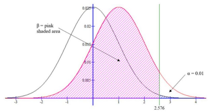
Two overlapping normal curves, a black curve centered at 0 and a red curve centered at 1, over an axis from −3 to 4. A green vertical line at 2.576 marks the critical value; the sliver of blue hatched area under the black curve to its right is labeled α = 0.01, and the large pink hatched area under the red curve to its left is labeled β = pink shaded area.

Figure 8-7

If we were to change $α$ from 0.05 to 0.01 then we get a critical value of $z sub α / 2$ = 2.576. Note that when $α$ decreases, then β increases which means your power 1 – β decreases. See Figure 8-7.

This text does not go over how to calculate β. You will need to be able to write out a sentence interpreting either the type I or II errors given a set of hypotheses. You also need to know the relationship between $α$ , β, confidence level, and power.

Hypothesis tests are not flawless, since we can make a wrong decision in statistical hypothesis tests based on the data. For example, in the court system, innocent people are sometimes wrongly convicted and the guilty sometimes walk free, or diagnostic tests that have false negatives or false positives. However, the difference is that in statistical hypothesis tests, we have the tools necessary to quantify how often we make such errors. A type I Error is rejecting the null hypothesis when H₀ is actually true. A type II Error is failing to reject the null hypothesis when the alternative is actually true (H₀ is false).

We use the symbols $α$ = P(Type I Error) and β = P(Type II Error). The critical value is a cutoff point on the horizontal axis of the sampling distribution that you can compare your test statistic to see if you should reject the null hypothesis. For a left-tailed test the critical value will always be on the left side of the sampling distribution, the right-tailed test will always be on the right side, and a two-tailed test will be on both tails. Use technology to find the critical values. Most of the time in this course the shortcut menus that we use will give you the critical values as part of the output.

8.2.1 Finding Critical Values

A researcher decides they want to have a 5% chance of making a type I error so they set α = 0.05. What z-score would represent that 5% area? It would depend on if the hypotheses were a left-tailed, two-tailed or right-tailed test. This z-score is called a critical value. Figure 8-8 shows examples of critical values for the three possible sets of hypotheses.

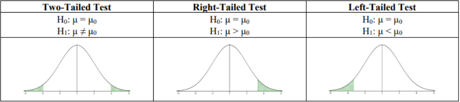
Figure 8-8

Two-tailed Test

If we are doing a two-tailed test then the $α$ = 5% area gets divided into both tails. We denote these critical values $z sub α / 2$ and $z sub 1 minus α / 2$ . When the sample data finds a z-score (test statistic) that is either less than or equal to $z sub α / 2$ or greater than or equal to $z sub 1 minus α / 2$ then we would reject H₀. The area to the left of the critical value $z sub α / 2$ and to the right of the critical value $z sub 1 minus α / 2$ is called the critical or rejection region. See Figure 8-9.

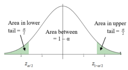
Standard normal curve with both tails shaded green, bounded on the left by z sub α/2 and on the right by z sub 1−α/2; labels read area in lower tail = α/2, area in upper tail = α/2, and area between = 1 − α.

Figure 8-9

When $α$ = 0.05 then the critical values $z sub α / 2$ and $z sub 1 minus α / 2$ are found using the following technology.

Excel: $z sub α / 2$ =NORM.S.INV(0.025) = –1.96 and $z sub 1 minus α / 2$ =NORM.S.INV(0.975) = 1.96

TI-Calculator: $z sub α / 2$ = invNorm(0.025,0,1) = –1.96 and $z sub 1 minus α / 2$ = invNorm(0.975,0,1) = 1.96

Since the normal distribution is symmetric, you only need to find one side’s z-score and we usually represent the critical values as ± $z sub α / 2$ .

Most of the time we will be finding a probability (p-value) instead of the critical values. The p-value and critical values are related and tell the same information so it is important to know what a critical value represents.

Right-tailed Test

If we are doing a right-tailed test then the $α$ = 5% area goes into the right tail. We denote this critical value $z sub 1 minus α$ . When the sample data finds a z-score more than $z sub 1 minus α$ then we would reject H₀, reject H₀ if the test statistic is ≥ $z sub 1 minus α$ . The area to the right of the critical value $z sub 1 minus α$ is called the critical region. See Figure 8-10.

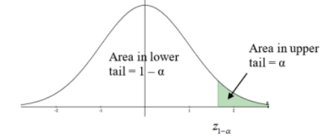
Normal curve with the upper tail beyond the critical value z sub 1−α shaded green; labels read area in lower tail = 1 − α and area in upper tail = α.

Figure 8-10

When $α$ = 0.05 then the critical value $z sub 1 minus α$ is found using the following technology.

Excel: $z sub 1 minus α$ =NORM.S.INV(0.95) = 1.645 Figure 8-10

TI-Calculator: $z sub 1 minus α$ = invNorm(0.95,0,1) = 1.645

Left-tailed Test

If we are doing a left-tailed test then the $α$ = 5% area goes into the left tail. If the sampling distribution is a normal distribution then we can use the inverse normal function in Excel or calculator to find the corresponding z-score. We denote this critical value $z_{α}$ .

When the sample data finds a z-score less than $z_{α}$ then we would reject H0, reject Ho if the test statistic is ≤ $z_{α}$ . The area to the left of the critical value $z_{α}$ is called the critical region. See Figure 8-11.

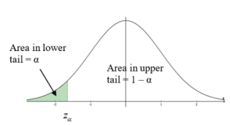
Normal curve with the lower tail below the critical value z sub α shaded green; labels read area in lower tail = α and area in upper tail = 1 − α.

Figure 8-11

When $α$ = 0.05 then the critical value $z_{α}$ is found using the following technology.

Excel: $z_{α}$ =NORM.S.INV(0.05) = –1.645

TI-Calculator: $z_{α}$ = invNorm(0.05,0,1) = –1.645

The Claim and Summary

The wording on the summary statement changes depending on which hypothesis the researcher claims to be true. We really should always be setting up the claim in the alternative hypothesis since most of the time we are collecting evidence to show that a change has occurred, but occasionally a textbook will have the claim in the null hypothesis. Do not use the phrase “accept H₀” since this implies that H0 is true. The lack of evidence is not evidence of nothing.

Caution! If we fail to reject the null this does not mean that there was no change, we just do not have any evidence that change has occurred. The absence of evidence is not evidence of absence. On the other hand, we need to be careful when we reject the null hypothesis we have not proved that there is change.

When we reject the null hypothesis, there is only evidence that a change has occurred. Our evidence could have been false and lead to an incorrect decision. If we use the phrase, “accept H₀” this implies that H₀ was true, but we just do not have evidence that it is false. Hence you will be marked incorrect for your decision if you use accept H₀, use instead “fail to reject H₀” or “do not reject H₀.”

Adapted from Mostly Harmless Statistics by Rachel Webb (Portland State University), hosted on LibreTexts (stats.libretexts.org) and licensed under CC BY-SA 4.0. Changes were made. License: CC-BY-SA-4.0.