7.5 Interpreting a Confidence Interval

There is always a chance that the confidence interval would not contain the true parameter that we are looking for. Inferential statistics does not “prove” that the population parameter is within the boundaries of the confidence interval. If the sample we took had all outliers and the sample statistic is far away from the true population parameter, then when we subtract and add the margin of error to the point estimate, the population parameter may not be within the limits.

Both the sample size and confidence level affect how wide the interval is. The following discussion demonstrates what happens to the width of the interval as you get more confident.

Think about shooting an arrow into the target. Suppose you are really good at that and that you have a 90% chance of hitting the bull’s-eye. Now the bull’s-eye is very small. Since you hit the bull’s eye approximately 90% of the time, then you probably hit inside the next ring out 95% of the time. You have a better chance of doing this, but the circle is bigger. You probably have a 99% chance of hitting the target, but that is a much bigger circle to hit. As your confidence in hitting the target increases, the circle you hit gets bigger. The same is true for confidence intervals.

The higher level of confidence makes a wider interval. There is a tradeoff between width and confidence level. You can be really confident about your answer, but your answer will not be very precise. On the other hand, you can have a precise answer (small margin of error) but not be very confident about your answer.

When we increase the confidence level, the confidence interval becomes wider to be more confident that the population parameter is within the lower and upper boundaries. A wider margin of error means less accuracy. When one is more confident, one would have a harder time predicting the true parameter with the larger range of values. See Figure 7-3.

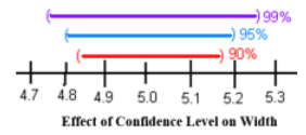
Figure 7-3

For instance, if we wanted to find the true mean grade for a statistics course using a 99% confidence critical value, we may get a very large margin of error, 75% ± 25%. This would say that we would be 99% confident that the average grade for all students is between 50% to 100%. This is of little help since that is anywhere between the grade range of F to an A. There are two ways to narrow this margin of error. The best way to reduce the margin of error is to increase the sample size, which decreases the standard deviation of the sampling distribution. When you take a larger sample, you will get a narrower interval. The other way to decrease the margin of error is to decrease your confidence level. When you decrease the confidence level, the critical value will be smaller. If we have a smaller margin of error then one can more accurately predict the population parameter.

Now look at how the sample size affects the size of the interval. Suppose the following Figure 7-4 represents confidence intervals calculated on a 95% interval.

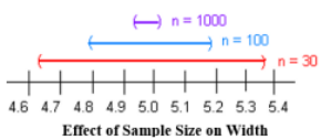
Figure 7-4

A larger sample size from a representative sample makes the standard error smaller and hence the width of the interval narrower. Large samples are closer to the true population so the point estimate is pretty close to the true value.

The following website is an applet where you can simulate confidence intervals with different parameters, sample sizes and confidence levels, take a moment and play around with the applet:

http://www.rossmanchance.com/applets/ConfSim.html.

The vertical bar in Figure 7-5 represents the true population mean test score of 75 (which would be unknown in real life). If you were to compute 100 confidence intervals using a 95% confidence level, then approximately 95/100 = 95% would contain the true population mean. The figure shows the confidence intervals as horizontal lines. There are 95 confidence intervals that contain the population mean shown in green. There are 5 confidence intervals that did not capture the population mean within the interval endpoints that are shown in red.

# Redraw Figure 7-5 live: 100 CIs at 95% around the true mean 75
# (sigma = 10 and n = 30 are demo choices; the book states only mu = 75)
set.seed(7)
mu <- 75; sigma <- 10; n <- 30
z <- qnorm(0.975)                      # z critical value -> 1.96
ci <- replicate(100, mean(rnorm(n, mu, sigma)) + c(-1, 1) * z * sigma / sqrt(n))
hit <- ci[1, ] <= mu & mu <= ci[2, ]
sum(hit)                               # about 95 of 100 intervals capture mu
plot(NA, xlim = range(ci), ylim = c(1, 100), xlab = "confidence interval", ylab = "sample")
segments(ci[1, ], 1:100, ci[2, ], 1:100, col = ifelse(hit, "green4", "red"))
abline(v = mu, lwd = 2)
# Figure 7-6: rerun with area 0.95 or 0.995 in qnorm(), and n <- 100

The probability that one confidence interval contains the mean is either zero or one. However, if we were to repeat the same sampling process, the proportion of times that the confidence intervals would capture the populations parameter is (1 – $\alpha$), where α is the complement of the confidence level. As an example, if you have a 95% confidence interval of 0.65 < p < 0.73, then you would say, “If we were to repeat this process, then 95% of the time the interval 0.65 to 0.73 would contain the true population proportion.” This means that if you have 100 intervals, 95 of them will contain the true proportion, and 5% will not.

The incorrect interpretation is that there is a 95% probability that the true value of p will fall between 0.65 and 0.73. The reason that this interpretation is incorrect is that the true value is fixed out there somewhere. You are trying to capture it with this interval. This is the chance that your interval captures the true mean, and not that the true value falls in the interval.

In addition, a real-world interpretation depends on the situation. It is where you are telling people what numbers you found the parameter to lie between. Therefore, your real-world interpretation is where you tell what values your parameter is between. There is no probability attached to this statement. That probability is in the statistical interpretation.

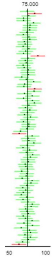
Figure 7-5

In the following Figure 7-6, confidence intervals were simulated using a 90% confidence level and then again using the 99% confidence level. Each confidence level was run 100 times with sample sizes of n = 30, then again using a sample size of n = 100, holding all other variables constant.

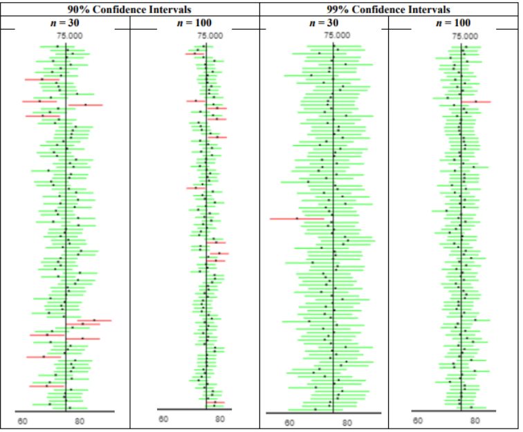
Figure 7-6

Compare columns 1 & 2 with columns 3 & 4 in Figure 7-6. For columns 1 & 2, 90/100 = 90% of the confidence intervals contain the mean. For columns 3 & 4, 99/100 = 99% of the confidence intervals contain the mean Note the higher confidence level is wider for the same sample size.

Compare columns 1 & 3 in Figure 7-6 and you can see that the width of the confidence interval is wider for the 99% confidence level compared to the 90% confidence level. Holding all other variables constant the confidence interval captured the population mean 99% of the time. Then compare columns 2 & 4 to see similar results.

The wider confidence intervals will more likely capture the true population mean, however you will have less accuracy in predicting what the true mean is.

“I'm not trying to prove anything, by the way. I'm a scientist and I know what constitutes proof. But the reason I call myself by my childhood name is to remind myself that a scientist must also be absolutely like a child. If he sees a thing, he must say that he sees it, whether it was what he thought he was going to see or not. See first, think later, then test. But always see first. Otherwise you will only see what you were expecting. Most scientists forget that.”

(Adams, 2002)

Adapted from Mostly Harmless Statistics by Rachel Webb (Portland State University), hosted on LibreTexts (stats.libretexts.org) and licensed under CC BY-SA 4.0. Changes were made. License: CC-BY-SA-4.0.