7.1 Introduction

Statistical inference is used to draw conclusions about a population based on a sample. We can use the probability distributions and Central Limit Theorem to understand what is going on in the population. The population can be difficult to measure so we take a sample from that population and use descriptive statistics to measure the sample. We can then use those sample statistics to infer back to what is happening in our population. Although there are many types of statistical inference tools, we will only cover some of the more common techniques.

Distinguishing between a population and a sample is important in statistics. We frequently use a representative sample to generalize a population.

A statistic is any characteristic or measure from a sample. One example is the sample mean $\bar{x}$ .
A parameter is any characteristic or measure from a population. One example is the population mean µ.
A point estimate for a parameter (a characteristic from a population) is a statistic (a characteristic from a sample). For example, the point estimate for the population mean µ is the sample mean $\bar{x}$ . The point estimate for the population standard deviation σ is the sample standard deviation s, etc.
A 100(1 – α)% confidence interval for a population parameter (μ, σ, etc.) represents that the proportion 100(1 – α)% of times the true value of the population parameter is contained within the interval.
The confidence level (or level of confidence) is 1 – α. The common percentages used for confidence interval levels are 90%, 95%, and 99%. Some corresponding values of alpha are: 90% would be α = 0.10 = 10%, 95% would be α = 0.05 = 5%, and 99% would be α = 0.01 = 1%. In this context, α, “alpha,” represents the complement of the confidence level, and its definition will be explained in the next chapter.

When a symmetric distribution, such as a normal distribution, is used, confidence intervals are always of the form: point estimate ± margin of error

The margin of error defines the “radius” of the interval necessary to obtain the desired confidence level. The margin of error depends on the desired confidence level. Higher levels of confidence come at a cost, namely larger margins of error, which means our estimate will be less accurate.

The margin of error formula will usually include a value from a sampling distribution called the critical value. The critical value measures the number of standard errors to be added and subtracted in order to achieve your desired confidence level based on the α level chosen.

For large sample sizes, the sampling distribution of a mean is normal. We can use the standard normal distribution values that would give the middle 95% of the distribution when α = 0.05 since 100(1 – 0.05)% = 95%.

The two critical values –z_α_/2 and +z_α_/2, as shown Figure 7-1. Note: in the notation z_α_/2 the α/2 represents the area in each of the tails.

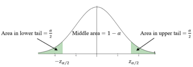
Standard normal curve with both tails shaded green and labeled: area in lower tail = α/2, middle area = 1 − α, and area in upper tail = α/2. The tail boundaries marked on the axis are −z α/2 and z α/2.

Figure 7-1

Assumption: If the sample size is small (n < 30), the population we are sampling from must be normal. If the sample size is “large” (n ≥ 30), the Central Limit Theorem guarantees that the sampling distribution will be normally distributed no matter how the population distribution is distributed.

Adapted from Mostly Harmless Statistics by Rachel Webb (Portland State University), hosted on LibreTexts (stats.libretexts.org) and licensed under CC BY-SA 4.0. Changes were made. License: CC-BY-SA-4.0.