4.2 Three Types of Probability
Classical Approach to Probability (Theoretical Probability)
The classical approach can only be used if each outcome has equal probability.
Empirical Probability (Experimental or Relative Frequency Probability)
The experiment is performed many times and the number of times that event A occurs is recorded. Then the probability is approximated by finding the relative frequency.
Definition
Important: The probability of any event A satisfies 0 ≤ P(A) ≤ 1, keep this in mind if the question is asking for a probability, and make sure your answer is a number between 0 and 1. A probability, relative frequency, percentage, and proportion are all different words for the same concept. Probability answers can be given as percentages, decimals, or reduced fractions.
Example 4
Suppose that the experiment is rolling a die. Compute the probability of rolling a 4.
Show solution
The sample space is S = {1, 2, 3, 4, 5, 6}. The event A is that you want is to get a 4, and the event space is A = {4}. To do this, roll a die 10 times. When you do that, you get 4 two times. Based on this experiment, the probability of getting a 4 is 2 out of 10 or 1/5 = 0.2. To get more accuracy, repeat the experiment more times. It is easiest to put this information in a table, where n represents the number of times the experiment is repeated. When you put the number of 4s found divisible by the number of times you repeat the experiment, this is the relative frequency. See the last column in Figure 4-3.
Figure 4-3: Trials for Die Experiment n Number of 4s Relative Frequency 10 2 0.2 50 6 0.12 100 18 0.18 500 81 0.162 1,000 163 0.163
Notice that as n increased, the relative frequency seems to approach a number; it looks like it is approaching 0.163. You can say that the probability of getting a 4 is approximately 0.163. If you want more accuracy, then increase n even more by rolling the die more times.
Try it in XYZ Crunch
Plot the Law of Large Numbers
Opens the Plots panel with Figure 4-3's trial sizes in L1 and the observed relative frequencies in L2. Pick the Scatter Plot tab (X = L1, Y = L2) and watch the points settle toward the theoretical probability 1/6 = 0.1667 as n grows.
These probabilities are called experimental probabilities since they are found by actually doing the experiment or simulation. They come about from the relative frequencies and give an approximation of the true probability.
The approximate probability of an event , notated as , is
For the event of getting a 4, the probability would be P(Roll a 4) = = 0.163
“‘What was that voice?’ shouted Arthur.
‘I don't know,’ yelled Ford, ‘I don't know. It sounded like a measurement of probability.’
‘Probability? What do you mean?’
‘Probability. You know, like two to one, three to one, five to four against. It said two to the power of one hundred thousand to one against. That's pretty improbable you know.’”
(Adams, 2002)
Definition
Law of Large Numbers: as n increases, the relative frequency tends towards the theoretical probability
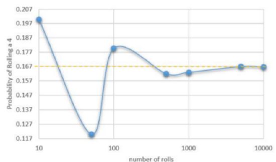
Figure 4-4 shows a graph of experimental probabilities as n gets larger and larger. The dashed yellow line is the theoretical probability of rolling a four of 1/6 0.1667. Note the x-axis is in a log scale.
# Roll a die 1,000 times and track the running relative frequency of a 4
set.seed(1)
rolls <- sample(1:6, 1000, replace = TRUE)
relfreq <- cumsum(rolls == 4) / seq_along(rolls)
relfreq[c(10, 50, 100, 500, 1000)] # the book's own rolls (Figure 4-3) gave 0.2, 0.12, 0.18, 0.162, 0.163
plot(relfreq, type = "l", log = "x", xlab = "n (log scale)",
ylab = "Relative frequency of a 4")
abline(h = 1/6, lty = 2, col = "red") # theoretical probability 1/6 = 0.1667
# Change the seed or the number of rolls -- every run drifts toward 1/6
Note that the more times you roll the die, the closer the experimental probability gets to the theoretical probability.

Figure 4-4
You can compute experimental probabilities whenever it is not possible to calculate probabilities using other means. An example is if you want to find the probability that a family has 5 children, you would have to actually look at many families, and count how many have 5 children. Then you could calculate the probability. Another example is if you want to figure out if a die is fair. You would have to roll the die many times and count how often each side comes up. Make sure you repeat an experiment many times, because otherwise you will not be able to estimate the true probability of 5 children. This is due to the law of large numbers, since the more times we repeat the experiment, the closer the experimental probabilities will get to the theoretical probabilities. For difficult theoretical probabilities, we can run computer simulations that can run an experiment repeatedly many times very quickly and come up with accurate estimates of the theoretical probability.
Example 5
A fitness center coach kept track of members over the last year. They recorded if the person stretched before they exercised, and whether they sustained an injury. The following contingency table shows their results. Select one member at random and find the following probabilities.
Injury
No Injury
Stretched
52 270
Did Not Stretch
21 57
- Compute the probability that a member sustained an injury.
- Compute the probability that a member did not stretch.
- Compute the probability that a member sustained an injury and did not stretch.
Show solution
a) Find the totals for each row, column, and grand total.
| Injury | No Injury | Total | |
|---|---|---|---|
| Stretched | 52 | 270 | 322 |
| Did Not Stretch | 21 | 57 | 78 |
| Total | 73 | 327 | 400 |
Next, find the relative frequencies by dividing each number by the total of 400.
| Injury | No Injury | Total | |
|---|---|---|---|
| Stretched | 0.13 | 0.675 | 0.805 |
| Did Not Stretch | 0.0525 | 0.1425 | 0.195 |
| Total | 0.1825 | 0.8175 | 1 |
Using the definition of a probability we get P(Injury) = = = 0.1825.
| Injury | No Injury | Total | |
|---|---|---|---|
| Stretched | 0.13 | 0.675 | 0.805 |
| Did Not Stretch | 0.0525 | 0.1425 | 0.195 |
| Total | 0.1825 | 0.8175 | 1 |
Using the table, we can get the same answer very quickly by just taking the column total under Injury to get 0.1825. As we get more complicated probability questions, these contingency tables will help organize your data.
b) Using the relative frequency contingency table, take the total of the row for all the members that did not stretch and we get the P(Did Not Stretch) = 0.195.
| Injury | No Injury | Total | |
|---|---|---|---|
| Stretched | 0.13 | 0.675 | 0.805 |
| Did Not Stretch | 0.0525 | 0.1425 | 0.195 |
| Total | 0.1825 | 0.8175 | 1 |
c) Using the relative frequency contingency table, take the intersection of the injury column with the did not stretch row and we get P(Injury and Did Not Stretch) = 0.0525.
| Injury | No Injury | Total | |
|---|---|---|---|
| Stretched | 0.13 | 0.675 | 0.805 |
| Did Not Stretch | 0.0525 | 0.1425 | 0.195 |
| Total | 0.1825 | 0.8175 | 1 |
3. Subjective Probability
The probability of event A is estimated using previous knowledge and is someone’s opinion.
Example 6
Compute the probability of meeting Dolly Parton.
Show solution
I estimate the probability of meeting Dolly Parton to be 1.2E-9 0.0000000012 (i.e. very, very small).
Example 7
What is the probability it will rain tomorrow?
Show solution
A weather reporter looks at several forecasts, uses their expert knowledge of the region, and reports the probability that it will rain in Portland, OR, is 80%.

Adapted from Mostly Harmless Statistics by Rachel Webb (Portland State University), hosted on LibreTexts (stats.libretexts.org) and licensed under CC BY-SA 4.0. Changes were made. License: CC-BY-SA-4.0.