1.9 First Order Linear PDE

We only considered ODE so far, so let us solve a linear first order PDE. Consider the equation

$a (x, t) u_{x} + b (x, t) u_{t} + c (x, t) u = g (x, t), u (x, 0) = f (x), - \infty < x < \infty, t > 0,$

where

u (x, t)

is a function of

x

and

t

. The initial condition

u open parenthesis x, 0 close parenthesis equals f open parenthesis x close parenthesis

is now a function of

x

rather than just a number. In these problems, it is useful to think of

x

as position and

t

as time. The equation describes the evolution of a function of

x

as time goes on. Below, the coefficients

a

b

c

, and the function

g

are mostly going to be constant or zero. The method we describe works with nonconstant coefficients, although the computations may get difficult quickly.

This method we use is the. The idea is that we find lines along which the equation is an ODE that we solve. We will see this technique again for second order PDE when we encounter the wave equation in Section 4.8.

Example 1

Consider the equation

$u_{t} + α u_{x} = 0, u (x, 0) = f (x) .$

This particular equation,

u_{t} + α u_{x} = 0

, is called the transport equation.

The data will propagate along curves called characteristics. The idea is to change to the so-called characteristic coordinates. If we change to these coordinates, the equation simplifies. The change of variables for this equation is

$ξ = x - α t, s = t .$

Let’s see what the equation becomes. Remember the chain rule in several variables.

$\begin{matrix} u_{t} = u_{ξ} ξ_{t} + u_{s} s_{t} = - α u_{ξ} + u_{s}, \\ u_{x} = u_{ξ} ξ_{x} + u_{s} s_{x} = u_{ξ} . \end{matrix}$

The equation in the coordinates $ξ$ and $s$ becomes

$\underset{u_{t}}{\underset{⏟}{(- α u_{ξ} + u_{s})}} + α \underset{u_{x}}{\underset{⏟}{(u_{ξ})}} = 0,$

or in other words

$u sub s equals 0.$

That is trivial to solve. Treating $ξ$ as simply a parameter, we have obtained the ODE $\frac{d u}{d s} = 0$ .

The solution is a function that does not depend on $s$ (but it does depend on $ξ$ ). That is, there is some function $A$ such that

$u = A (ξ) = A (x - α t) .$

The initial condition says that:

$f (x) = u (x, 0) = A (x - α 0) = A (x),$

A = f

. In other words,

$u (x, t) = f (x - α t) .$

Everything is simply moving right at speed

α

t

increases. The curve given by the equation

$ξ = constant$

is called the characteristic. See Figure $1$ . In this case, the solution does not change along the characteristic.

Figure

1

: Characteristic curves.

In the $(x, t)$ coordinates, the characteristic curves satisfy $t = \frac{1}{α} (x - ξ)$ , and are in fact lines. The slope of characteristic lines is $\frac{1}{α}$ , and for each different $ξ$ we get a different characteristic line.

We see why $u_{t} + α u_{x} = 0$ is called the transport equation: everything travels at some constant speed. Sometimes this is called. An example application is material being moved by a river where the material does not diffuse and is simply carried along. In this setup, $x$ is the position along the river, $t$ is the time, and $u (x, t)$ the concentration the material at position $x$ and time $t$ . See Figure $2$ for an example.

Figure

2

: Example of “transport” in

u_{t} - u_{x} = 0

(that is,

α equals 1

) where the initial condition

f (x)

is a peak at the origin. On the left is a graph of the initial condition

u open parenthesis x, 0 close parenthesis

. On the right is a graph of the function

u open parenthesis x, 1 close parenthesis

, that is at time

t equals 1

. Notice it is the same graph shifted one unit to the right.

We use similar idea in the more general case:

$a u_{x} + b u_{t} + c u = g, u (x, 0) = f (x) .$

We change coordinates to the characteristic coordinates. Let us call these coordinates

(ξ, s)

. These are coordinates where

a u_{x} + b u_{t}

becomes differentiation in the

s

variable.

Along the characteristic curves (where $ξ$ is constant), we get a new ODE in the $s$ variable. In the transport equation, we got the simple $\frac{d u}{d s} = 0$ . In general, we get the linear equation

$\frac{d u}{d s} + c u = g .$

(1.9.1)

We think of everything as a function of $ξ$ and $s$ , although we are thinking of $ξ$ as a parameter rather than an independent variable. So the equation is an ODE. It is a linear ODE that we can solve using the integrating factor.

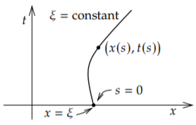
To find the characteristics, think of a curve given parametrically $(x (s), t (s))$ . We try to have the curve satisfy

$\frac{d x}{d s} = a, \frac{d t}{d s} = b .$

Why? Because when we think of

x

and

t

as functions of

s

we find, using the chain rule,

$\frac{d u}{d s} + c u = \underset{\frac{d u}{d s}}{\underset{⏟}{(u_{x} \frac{d x}{d s} + u_{t} \frac{d t}{d s})}} + c u = a u_{x} + b u_{t} + c u = g .$

So we get the ODE (1.9.1), which then describes the value of the solution $u$ of the PDE along this characteristic curve. It is also convenient to make sure that $s equals 0$ corresponds to $t equals 0$ , that is $t open parenthesis 0 close parenthesis equals 0$ . It will be convenient also for $x open parenthesis 0 close parenthesis equals ξ$ . See Figure $3$ .

The graph contains (epsilon,0) at x=0 and goes through (x(s),t(s)). — Figure $3$ : General characteristic curve.

Example 2

Consider

$u_{x} + u_{t} + u = x, u (x, 0) = e^{- x^{2}} .$

We find the characteristics, that is, the curves given by

$\frac{d x}{d s} = 1, \frac{d t}{d s} = 1 .$

$x = s + c_{1}, t = s + c_{2},$

for some

c sub 1

and

c sub 2

. At

s equals 0

we want

t equals 0

, and

x

should be

ξ

. So we let

c sub 1 equals ξ

and

c sub 2 equals 0

$x = s + ξ, t = s .$

The ODE is $\frac{d u}{d s} + u = x$ , and $x = s + ξ$ . So, the ODE to solve along the characteristic is

$\frac{d u}{d s} + u = s + ξ .$

The general solution of this equation, treating

ξ

as a parameter, is

u = C e^{- s} + s + ξ - 1

, for some constant

C

. At

s equals 0

, our initial condition is that

u

e^{- ξ^{2}}

, since at

s equals 0

we have

x = ξ

. Given this initial condition, we find

C = e^{- ξ^{2}} - ξ + 1

. So,

$\begin{matrix} u = (e^{- ξ^{2}} - ξ + 1) e^{- s} + s + ξ - 1 \\ = e^{- ξ^{2} - s} + (1 - ξ) e^{- s} + s + ξ - 1 . \end{matrix}$

Substitute $ξ = x - t$ and $s = t$ to find $u$ in terms of $x$ and $t$ :

$\begin{matrix} u = e^{- ξ^{2} - s} + (1 - ξ) e^{- s} + s + ξ - 1 \\ = e^{- {(x - t)}^{2} - t} + (1 - x + t) e^{- t} + x - 1 . \end{matrix}$

See Figure

4

for a plot of

u (x, t)

as a function of two variables.

The section's worked solution u = e^(−(x−t)²−t) + (1 − x + t)e^(−t) + x − 1, drawn as a profile in x instead of a frozen 3D surface. Drag t: at t = 0 the curve is exactly the initial condition e^(−x²), then the bump rides right at unit speed along the characteristics x − t = constant while the u term damps its height like e^(−t), and the whole profile relaxes onto the dashed steady state u = x − 1 forced by g = x.

Figure

4

: Plot of the solution

u (x, t)

u_{x} + u_{t} + u = x

u (x, 0) = e^{- x^{2}}

When the coefficients are not constants, the characteristic curves are not going to be straight lines anymore.

We make a few closing remarks. One thing to keep in mind is that we would get into trouble if the coefficient in front of $u_{t}$ , that is the $b$ , is ever zero. Let us consider a quick example of what can go wrong:

$u_{x} + u = 0, u (x, 0) = \sin (x) .$

This problem has no solution. If we had a solution, it would imply that

u sub x open parenthesis x, 0 close parenthesis equals cos open parenthesis x close parenthesis

, but

u_{x} (x, 0) + u (x, 0) = \cos (x) + \sin (x) ⧸ = 0

. The problem is that the characteristic curve is now the line

t equals 0

, and the solution is already provided on that line!

As long as $b$ is nonzero, it is convenient to ensure that $b$ is positive by multiplying by $minus 1$ if necessary, so that positive $s$ means positive $t$ .

Another remark is that if $a$ or $b$ in the equation are variable, the computations can quickly get out of hand, as the expressions for the characteristic coordinates become messy and then solving the ODE becomes even messier. In the examples above, $b$ was always $1$ , meaning we got $s = t$ in the characteristic coordinates. If $b$ is not constant, your expression for $s$ will be more complicated.

Finding the characteristic coordinates is really a system of ODE in general if $a$ depends on $t$ or if $b$ depends on $x$ . In that case, we would need techniques of systems of ODE to solve, see Chapter 3 or Chapter 8. In general, if $a$ and $b$ are not linear functions or constants, finding closed form expressions for the characteristic coordinates may be impossible.

Finally, the method of characteristics applies to nonlinear first order PDE as well. In the nonlinear case, the characteristics depend not only on the differential equation, but also on the initial data. This leads to not only more difficult computations, but also the formation of singularities where the solution breaks down at a certain point in time. An example application where first order nonlinear PDE come up is traffic flow theory, and you have probably experienced the formation of singularities: traffic jams. But we digress.

Adapted from Differential Equations for Engineers by Jiří Lebl (Oklahoma State University), hosted on LibreTexts (math.libretexts.org) and licensed under CC BY-SA 4.0. Changes were made. License: CC-BY-SA-4.0.