Differential Equations for EngineersXYZ Homework Edition

⇩ Download ▾

1.5 Substitution

Just as when solving integrals, one method to try is to change variables to end up with a simpler equation to solve.

Substitution

The equation

y = ( x y + 1 ) 2 y' = (x-y + 1)^2 \label{1.5.1}

(1.5.1)

is neither separable nor linear. What can we do? How about trying to change variables, so that in the new variables the equation is simpler. We use another variable vv, which we treat as a function of xx. Let us try

v = x y + 1 . v=x-y+1. \label{1.5.2}

(1.5.2)

We need to figure out yy' in terms of vv', vv and xx. We differentiate (in xx) to obtain v=1yv' = 1 -y'. So y=1vy' = 1 - v'. We plug this into the equation to get

1 v = v 2 1 - v' = v^2 \label{1.5.3}

(1.5.3)

In other words, v=1v2v' = 1 - v^2. Such an equation we know how to solve by separating variables:

1 1 v 2 d v = d x \dfrac {1}{1 -v^2} dv = dx \label{1.5.5}

(1.5.4)

So

1 2 ln | v + 1 v 1 | = x + C , or | v + 1 v 1 | = e 2 x + 2 C , or v + 1 v 1 = D e 2 x , \frac{1}{2}\ln\left|\frac{v+1}{v-1}\right| =x+C,\quad\text{or}\quad\left|\frac{v+1}{v-1}\right|=e^{2x+2C},\quad\text{or}\quad\frac{v+1}{v-1}=De^{2x}, \nonumber

for some constant DD. Note that v=1v = 1 and v=1v = -1 are also solutions.

Now we need to “unsubstitute” to obtain

x y + 2 x y = D e 2 x \dfrac {x - y + 2}{x -y} = De^{2x} \label{1.5.8}

(1.5.5)

and also the two solutions xy+1=1x - y + 1 = 1 or y=xy = x, and xy+1=1x - y + 1 = -1 or y=x+2y = x + 2. We solve the first equation for yy.

x y + 2 = ( x y ) D e 2 x , x y + 2 = D x e 2 x y D e 2 x , y + y D e 2 x = D x e 2 x x 2 , y ( 1 + D e 2 x ) = D x e 2 x x 2 , y = D x e 2 x x 2 D e 2 x 1 . \begin{align}\begin{aligned} x - y + 2 &= \left ( x - y \right ) De^{2x}, \\ x - y + 2 &= Dxe^{2x} - yDe^{2x}, \\ -y + yDe^{2x} &= Dxe^{2x} - x - 2, \\ y( -1 + De^{2x}) &= Dxe^{2x} - x - 2, \\ y &= \dfrac {Dxe^{2x} - x - 2}{De^{2x} - 1}.\end{aligned}\end{align} \nonumber

Note that D=0D = 0 gives y=x+2y = x + 2, but no value of DD gives the solution y=xy = x.

Substitution in differential equations is applied in much the same way that it is applied in calculus. You guess. Several different substitutions might work. There are some general things to look for. We summarize a few of these in a table.

When you see Try substituting
y y yy' v = y 2 v = y^2
y 2 y y^2y' v = y 3 v = y^3
( cos y ) y (\cos y )y' v = sin y v = \sin y
( sin y ) y (\sin y )y' v = cos y v = \cos y
y e y y'e^y v = e y v = e^y

Usually you try to substitute in the “most complicated” part of the equation with the hopes of simplifying it. The above table is just a rule of thumb. You might have to modify your guesses. If a substitution does not work (it does not make the equation any simpler), try a different one.

Bernoulli Equations

There are some forms of equations where there is a general rule for substitution that always works. One such example is the so-called Bernoulli equation.1

y + p ( x ) y = q ( x ) y n y' + p(x)\,y = q(x)\, y^n \label{1.5.15}

(1.5.6)

This equation looks a lot like a linear equation except for the yny^n. If n=0n = 0 or n=1n =1, then the equation is linear and we can solve it. Otherwise, the substitution v=y1nv = y^{1 - n} transforms the Bernoulli equation into a linear equation. Note that nn need not be an integer.

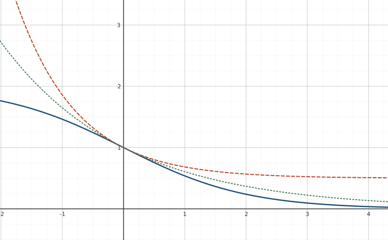
Interactive figureBernoulli equation y′ + y = ½yⁿ, with n on a sliderDrag the Bernoulli exponent n slider from -2 to 4.
Three curves cross at a single point one unit above the origin, where a shared starting value pins them, and all fall away to the right. The solid curve is the one the slider controls; the two dashed curves are the linear cases the section names, and neither moves. At the default setting the solid curve runs below both everywhere except at that shared point: it enters from the left at a modest height while the other two drop in steeply, one of them from above the top edge, and it sinks onto the horizontal axis first, near the right-hand edge. Raising the exponent flattens its left arm and presses its tail harder onto the axis; lowering it swings that arm into a steep climb off the top of the frame and lifts the tail clear of it instead. At exponent zero the solid curve vanishes beneath the long-dashed one, the two lying exactly together. Adjustable parameter: Bernoulli exponent n (n) = 2. Viewing window: x from -2.02 to 4.32, y from -0.51 to 3.41.
XYZ Graph · viewer build 5edf91b
A Bernoulli equation with constant coefficients, y′ + y = ½yⁿ, started from y(0) = 1 and solved by this section's own substitution v = y¹⁻ⁿ: y = ((1 + e^(-(1-n)x))/2)^(1/(1-n)). Every member of the family leaves the same point, so the exponent alone decides the shape. The two fixed curves are the cases the text calls out. The long-dashed one is n = 0, where v = y¹⁻ⁿ is just v = y — the substitution changes nothing, and dragging n there lays the solid curve exactly on top of it. The finely dotted one is n = 1, where that same substitution collapses to v = 1 and records nothing about y at all; the exponent 1/(1 - n) blows up with it, which is why the slider steps over n = 1 rather than through it. The equation is still linear there, and the dotted curve is its solution, e^(-x/2). That curve is also the boundary between the two behaviours: below n = 1 the solution settles at a positive level, above it the solution decays to zero, and the settling level itself falls toward zero as n rises to 1, which is how the two sides meet. n need not be an integer, so the slider moves in steps of 0.4.

v 4 ( x + 1 ) x v = 4 v' - \dfrac {4(x + 1)}{x} v = 4 \nonumber

Now the equation is linear. We can use the integrating factor method. In particular, we use formula (1.4.17). Let us assume that x>0x > 0 so |x|=x\left \vert x \right \vert = x. This assumption is OK, as our initial condition is x=1x = 1. Let us compute the integrating factor. Here p(s)p(s) from formula (1.4.17) is 4(s+1)s\dfrac {-4(s + 1)}{s}.

e 1 x p ( s ) d s = exp ( 1 x 4 ( s + 1 ) s d s ) = e 4 x 4 l n ( x ) + 4 = e 4 x + 4 x 4 = e 4 x + 4 x 4 , e 1 x p ( s ) d s = e 4 x + 4 l n ( x ) 4 = e 4 x 4 x 4 \begin{align}\begin{aligned} e^{\int _1^x p(s) ds} &= \text {exp} \left ( \int ^x_1 \dfrac {-4(s + 1)}{s} ds \right ) = e^{-4x - 4ln(x) + 4} = e^{-4x + 4} x^{-4} = \dfrac {e^{-4x + 4}}{x^4}, \\ e^{- \int_1^x p(s) ds} &= e^{4x + 4ln(x) - 4} = e^{4x - 4} x^4\end{aligned}\end{align} \nonumber

We now plug in to (1.4.17)

v ( x ) = e 1 x p ( s ) d s ( 1 x e 1 t p ( s ) d s 4 d t + 1 ) , = e 4 x 4 x 4 ( 1 x 4 e 4 t + 4 t 4 d t + 1 ) \begin{align}\begin{aligned} v(x) &= e^{- \int_1^x p(s)ds} \left ( \int_1^x e^{\int_1^t p(s)ds} 4 dt + 1\right ), \\ &= e^{4x - 4} x^4 \left ( \int_1^x 4 \dfrac {e^{-4t+4}}{t^4} dt + 1 \right ) \end{aligned}\end{align} \nonumber

Note that the integral in this expression is not possible to find in closed form. As we said before, it is perfectly fine to have a definite integral in our solution. Now “unsubstitute”

y 4 = e 4 x 4 x 4 ( 4 1 x e 4 t + 4 t 4 d t + 1 ) , y = e x + 1 x ( 4 1 x e 4 t + 4 t 4 d t + 1 ) 1 / 4 \begin{align}\begin{aligned} y^{-4} &= e^{4x - 4} x^{4} \left ( 4 \int_1^x \dfrac {e^{-4t + 4}}{t^4} dt + 1 \right ), \\ y &= \dfrac {e^{-x+1}}{x \left (4 \int_1^x \dfrac {e^{-4t+4}}{t^4} dt + 1\right )^{1/4}} \end{aligned}\end{align} \nonumber

Homogeneous Equations

Another type of equations we can solve by substitution are the so-called homogeneous equations. Suppose that we can write the differential equation as

y = F ( y x ) y' = F \left ( \dfrac {y}{x} \right ) \label{1.5.16}

(1.5.7)

Here we try the substitutions

v = y x and therefore y = v + x v v = \dfrac {y}{x} \quad\text{and therefore}\quad y' = v + xv' \label{1.5.17}

(1.5.8)

We note that the equation is transformed into

v + x v = F ( v ) or x v = F ( v ) v or v F ( v ) v = 1 x v + xv' = F(v) \quad\text{or}\quad xv' = F(v) - v \quad\text{or}\quad \dfrac {v'}{F(v) - v} = \dfrac {1}{x} \label{1.5.18}

(1.5.9)

Hence an implicit solution is

1 F ( v ) v d v = ln | x | + C \int \dfrac {1}{F(v) - v} dv = \ln \left \vert x \right \vert + C \label{1.5.19}

(1.5.10)

Footnotes

[1] There are several things called Bernoulli equations, this is just one of them. The Bernoullis were a prominent Swiss family of mathematicians. These particular equations are named for Jacob Bernoulli (1654–1705).

Adapted from Differential Equations for Engineers by Jiří Lebl (https://www.jirka.org/diffyqs/), © Jiří Lebl, licensed under CC BY-SA 4.0. Changes were made. License: CC-BY-SA-4.0.

These eBooks are a prerelease and are not yet certified conformant with WCAG 2.1 AA or ADA Title II. Every page is built against an automated accessibility gate, and the published editions will meet ADA Title II requirements when they release in late September 2026. If something is unusable, please tell us.