1.8 Exact Equations

Another type of equation that comes up quite often in physics and engineering is an exact equation. Suppose $F (x, y)$ is a function of two variables, which we call the potential function. The naming should suggest potential energy, or electric potential. Exact equations and potential functions appear when there is a conservation law at play, such as conservation of energy. Let us make up a simple example. Let

$F (x, y) = x^{2} + y^{2} .$

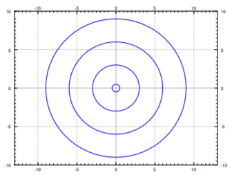
We are interested in the lines of constant energy, that is lines where the energy is conserved; we want curves where $F (x, y) = C$ , for some constant $C$ . In our example, the curves $x^{2} + y^{2} = C$ are circles. See Figure $1$ .

Plot of four concentric blue circles centred on the origin, radii roughly 0.5, 3, 6 and 9, on axes about -13 to 13 by -10 to 10. They nest as closed level curves without touching. — Figure $1$ : Solutions to $F (x, y) = x^{2} + y^{2} = C$ for various $C$ .

We take the total derivative of $F$ :

$d F = \frac{\partial F}{\partial x} d x + \frac{\partial F}{\partial y} d y .$

For convenience, we will make use of the notation of $F_{x} = \frac{\partial F}{\partial x}$ and $F_{y} = \frac{\partial F}{\partial y}$ . In our example,

$d F = 2 x d x + 2 y d y .$

We apply the total derivative to $F (x, y) = C$ , to find the differential equation $d F equals 0$ . The differential equation we obtain in such a way has the form

$M d x + N d y = 0, or M + N \frac{d y}{d x} = 0 .$

An equation of this form is called exact if it was obtained as $d F equals 0$ for some potential function $F$ . In our simple example, we obtain the equation

$2 x d x + 2 y d y = 0, or 2 x + 2 y \frac{d y}{d x} = 0 .$

Since we obtained this equation by differentiating $x^{2} + y^{2} = C$ , the equation is exact. We often wish to solve for $y$ in terms of $x$ . In our example,

$y = \pm \sqrt{C^{2} - x^{2}} .$

An interpretation of the setup is that at each point $\vec{v} = (M, N)$ is a vector in the plane, that is, a direction and a magnitude. As $M$ and $N$ are functions of $(x, y)$ , we have a vector field. The particular vector field $\vec{v}$ that comes from an exact equation is a so-called conservative vector field, that is, a vector field that comes with a potential function $F (x, y)$ , such that

$\vec{v} = (\frac{\partial F}{\partial x}, \frac{\partial F}{\partial y}) .$

Let

γ

be a path in the plane starting at

open parenthesis x sub 1, y sub 1 close parenthesis

and ending at

open parenthesis x sub 2, y sub 2 close parenthesis

. If we think of

\vec{v}

as force, then the work required to move along

γ

$\int_{γ} \vec{v} (\vec{r}) \cdot d \vec{r} = \int_{γ} M d x + N d y = F (x_{2}, y_{2}) - F (x_{1}, y_{1}) .$

That is, the work done only depends on endpoints, that is where we start and where we end. For example, suppose $F$ is gravitational potential. The derivative of $F$ given by $\vec{v}$ is the gravitational force. What we are saying is that the work required to move a heavy box from the ground floor to the roof, only depends on the change in potential energy. That is, the work done is the same no matter what path we took; if we took the stairs or the elevator. Although if we took the elevator, the elevator is doing the work for us. The curves $F (x, y) = C$ are those where no work need be done, such as the heavy box sliding along without accelerating or breaking on a perfectly flat roof, on a cart with incredibly well oiled wheels.

An exact equation is a conservative vector field, and the implicit solution of this equation is the potential function.

Solving exact equations

Now you, the reader, should ask: Where did we solve a differential equation? Well, in applications we generally know $M$ and $N$ , but we do not know $F$ . That is, we may have just started with $2 x + 2 y \frac{d y}{d x} = 0$ , or perhaps even

$x + y \frac{d y}{d x} = 0 .$

It is up to us to find some potential $F$ that works. Many different $F$ will work; adding a constant to $F$ does not change the equation. Once we have a potential function $F$ , the equation $F (x, y (x)) = C$ gives an implicit solution of the ODE.

Example 1

Let us find the general solution to $2 x + 2 y \frac{d y}{d x} = 0$ . Forget we knew what $F$ was.

Show solution

If we know that this is an exact equation, we start looking for a potential function $F$ . We have $M equals 2 x$ and $N equals 2 y$ . If $F$ exists, it must be such that $F sub x open parenthesis x, y close parenthesis equals 2 x$ . Integrate in the $x$ variable to find

$F (x, y) = x^{2} + A (y),$

(1.8.1)

for some function $A (y)$ . The function $A$ is the "constant of integration," though it is only constant as far as $x$ is concerned, and may still depend on $y$ . Now differentiate (1.8.1) in $y$ and set it equal to $N$ , which is what $F_{y}$ is supposed to be:

$2 y = F_{y} (x, y) = A^{'} (y) .$

Integrating, we find $A (y) = y^{2}$ . We could add a constant of integration if we wanted to, but there is no need. We found $F (x, y) = x^{2} + y^{2}$ . Next for a constant $C$ , we solve

$F (x, y (x)) = C .$

for $y$ in terms of $x$ . In this case, we obtain $y = \pm \sqrt{C^{2} - x^{2}}$ as we did before.

The procedure, once we know that the equation is exact, is:

Integrate $F_{x} = M$ in $x$ resulting in $F (x, y) = something + A (y)$ .
Differentiate this $F$ in $y$ , and set that equal to $N$ , so that we may find $A (y)$ by integration.

The procedure can also be done by first integrating in $y$ and then differentiating in $x$ . Pretty easy huh? Let’s try this again.

Is there an easier way to check for the existence of $F$ , other than failing in trying to find it? Turns out there is. Suppose $M = F_{x}$ and $N = F_{y}$ . Then as long as the second derivatives are continuous,

$\frac{\partial M}{\partial y} = \frac{\partial^{2} F}{\partial y \partial x} = \frac{\partial^{2} F}{\partial x \partial y} = \frac{\partial N}{\partial x} .$

Let us state it as a theorem. Usually this is called the Poincaré Lemma.to the power 1

The theorem doesn’t give us a global $F$ defined everywhere. In general, we can only find the potential locally, near some initial point. By this time, we have come to expect this from differential equations.

Let us return to Example $2$ where $M = 2 x + y$ and $N = x y$ . Notice $M sub y equals 1$ and $N_{x} = y$ , which are clearly not equal. The equation is not exact.

Example 4

Solve

$- \frac{y}{x^{2} + y^{2}} d x + \frac{x}{x^{2} + y^{2}} d y = 0, y (1) = 2 .$

Show solution

We leave to the reader to check that $M_{y} = N_{x}$ .

This vector field $(M, N)$ is not conservative if considered as a vector field of the entire plane minus the origin. The problem is that if the curve $γ$ is a circle around the origin, say starting at $open parenthesis 1, 0 close parenthesis$ and ending at $open parenthesis 1, 0 close parenthesis$ going counterclockwise, then if $F$ existed we would expect

$0 = F (1, 0) - F (1, 0) = \int_{γ} F_{x} d x + F_{y} d y = \int_{γ} \frac{- y}{x^{2} + y^{2}} d x + \frac{x}{x^{2} + y^{2}} d y = 2 π .$

That is nonsense! We leave the computation of the path integral to the interested reader, or you can consult your multivariable calculus textbook. So there is no potential function $F$ defined everywhere outside the origin $open parenthesis 0, 0 close parenthesis$ .

If we think back to the theorem, it does not guarantee such a function anyway. It only guarantees a potential function locally, that is only in some region near the initial point. As $y open parenthesis 1 close parenthesis equals 2$ we start at the point $open parenthesis 1, 2 close parenthesis$ . Considering $x greater than 0$ and integrating $M$ in $x$ or $N$ in $y$ , we find

$F (x, y) = arctan (\frac{y}{x}) .$

The implicit solution is $arctan (\frac{y}{x}) = C$ . Solving, $y = \tan (C) x$ . That is, the solution is a straight line. Solving $y open parenthesis 1 close parenthesis equals 2$ gives us that $tan open parenthesis C close parenthesis equals 2$ , and so $y equals 2 x$ is the desired solution. See Figure $1$ , and note that the solution only exists for $x greater than 0$ .

Figure

1

: Solution to

- \frac{y}{x^{2} + y^{2}} d x + \frac{x}{x^{2} + y^{2}} d y = 0

y open parenthesis 1 close parenthesis equals 2

, with initial point marked.

Integrating factors

Sometimes an equation $M d x + N d y = 0$ is not exact, but it can be made exact by multiplying with a function $u (x, y)$ . That is, perhaps for some nonzero function $u (x, y)$ ,

$u (x, y) M (x, y) d x + u (x, y) N (x, y) d y = 0$

is exact. Any solution to this new equation is also a solution to

M d x + N d y = 0

In fact, a linear equation

$\frac{d y}{d x} + p (x) y = f (x), or (p (x) y - f (x)) d x + d y = 0$

is always such an equation. Let

r (x) = e^{\int p (x) d x}

be the integrating factor for a linear equation. Multiply the equation by

r (x)

and write it in the form of

M + N \frac{d y}{d x} = 0

$r (x) p (x) y - r (x) f (x) + r (x) \frac{d y}{d x} = 0 .$

Then

M = r (x) p (x) y - r (x) f (x)

, so

M_{y} = r (x) p (x)

, while

N = r (x)

, so

N_{x} = r^{'} (x) = r (x) p (x)

. In other words, we have an exact equation. Integrating factors for linear functions are just a special case of integrating factors for exact equations.

But how do we find the integrating factor $u$ ? Well, given an equation

$M d x + N d y = 0,$

u

should be a function such that

$\frac{\partial}{\partial y} [u M] = u_{y} M + u M_{y} = \frac{\partial}{\partial x} [u N] = u_{x} N + u N_{x} .$

Therefore,

$(M_{y} - N_{x}) u = u_{x} N - u_{y} M .$

At first it may seem we replaced one differential equation by another. True, but all hope is not lost.

A strategy that often works is to look for a $u$ that is a function of $x$ alone, or a function of $y$ alone. If $u$ is a function of $x$ alone, that is $u (x)$ , then we write $u^{'} (x)$ instead of $u_{x}$ , and $u_{y}$ is just zero. Then

$\frac{M_{y} - N_{x}}{N} u = u^{'} .$

In particular,

\frac{M_{y} - N_{x}}{N}

ought to be a function of

x

alone (not depend on

y

). If so, then we have a linear equation

$u^{'} - \frac{M_{y} - N_{x}}{N} u = 0 .$

Letting

P (x) = \frac{M_{y} - N_{x}}{N}

, we solve using the standard integrating factor method, to find

u (x) = C e^{\int P (x) d x}

. The constant in the solution is not relevant, we need any nonzero solution, so we take

C equals 1

. Then

u (x) = e^{\int P (x) d x}

is the integrating factor.

Similarly we could try a function of the form $u (y)$ . Then

$\frac{M_{y} - N_{x}}{M} u = - u^{'} .$

In particular,

\frac{M_{y} - N_{x}}{M}

ought to be a function of

y

alone. If so, then we have a linear equation

$u^{'} + \frac{M_{y} - N_{x}}{M} u = 0 .$

Letting

Q (y) = \frac{M_{y} - N_{x}}{M}

, we find

u (y) = C e^{- \int Q (y) d y}

. We take

C equals 1

. So

u (y) = e^{- \int Q (y) d y}

is the integrating factor.

Example 7

Solve

$y^{2} + (x y + 1) \frac{d y}{d x} = 0 .$

Show solution

First compute

$M_{y} - N_{x} = 2 y - y = y .$

As this is not zero, the equation is not exact. We observe

$Q (y) = \frac{M_{y} - N_{x}}{M} = \frac{y}{y^{2}} = \frac{1}{y}$

is a function of

y

alone. We compute the integrating factor

$e^{- \int Q (y) d y} = e^{- \ln y} = \frac{1}{y} .$

Therefore we look at the exact equation

$y + \frac{x y + 1}{y} \frac{d y}{d x} = 0 .$

The reader should double check that this equation is exact. We follow the procedure for exact equations

$F (x, y) = x y + A (y),$

and

$\frac{x y + 1}{y} = x + \frac{1}{y} = x + A^{'} (y) .$

Consequently

A^{'} (y) = \frac{1}{y}

A (y) = \ln y

. Thus

F (x, y) = x y + \ln y

. It is not possible to solve

F (x, y) = C

for

y

in terms of elementary functions, so let us be content with the implicit solution:

$x y + \ln y = C .$

We are looking for the general solution and we divided by

y

above. We should check what happens when

y equals 0

, as the equation itself makes perfect sense in that case. We plug in

y equals 0

to find the equation is satisfied. So

y equals 0

is also a solution.

Footnotes

[1] Named for the French polymath Jules Henri Poincaré (1854–1912).

Adapted from Differential Equations for Engineers by Jiří Lebl (Oklahoma State University), hosted on LibreTexts (math.libretexts.org) and licensed under CC BY-SA 4.0. Changes were made. License: CC-BY-SA-4.0.