Differential Equations for EngineersXYZ Homework Edition

⇩ Download ▾

1.6 Autonomous equations

Let us consider general differential equation problems of the form

d x d t = f ( x ) \dfrac{dx}{dt} = f(x) \nonumber

where the derivative of solutions depends only on xx (the dependent variable). Such equations are called autonomous equations. If we think of tt as time, the naming comes from the fact that the equation is independent of time.

Let us come back to the cooling coffee problem (see Example 1.3.3). Newton’s law of cooling says that

d x d t = k ( x A ) \dfrac{dx}{dt} = -k(x-A) \nonumber

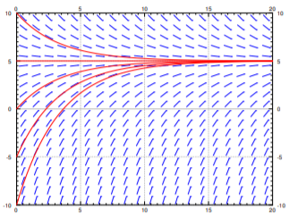
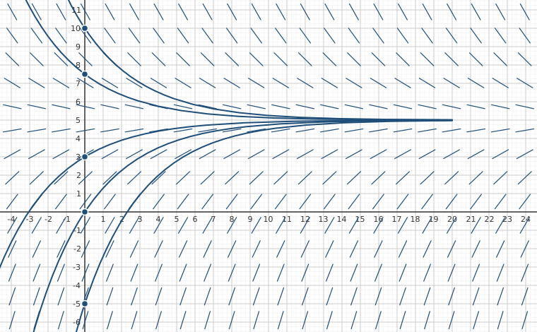
where xx is the temperature, tt is time, kk is some constant, and AA is the ambient temperature. See Figure 1\PageIndex{1} for an example with k=0.3k = 0.3 and A=5A = 5.

Note the solution x=Ax = A (in the figure x=5x = 5). We call these constant solutions the equilibrium solutions. The points on the xx axis where f(X)=0f(X) = 0 are called critical points. The point x=Ax = A is a critical point. In fact, each critical point corresponds to an equilibrium solution. Note also, by looking at the graph, that the solution x=Ax = A is “stable” in that small perturbations in xx do not lead to substantially different solutions as tt grows. If we change the initial condition a little bit, then as tt \rightarrow \infty we get xAx \rightarrow A. We call such critical points stable. In this simple example it turns out that all solutions in fact go to AA as tt \rightarrow \infty. If a critical point is not stable we would say it is unstable.
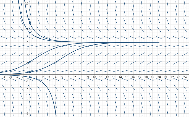
Interactive figureSlope field for x′ = k(5 − x): the rate sets how fast solutions reach the equilibriumDrag the Rate k slider from 0 to 1.2.
Short slope segments fill the frame with time running left to right. They lie flat along one horizontal level partway up, tilt upward everywhere below it and downward everywhere above, more steeply the further away. Five solution curves start at different heights, above and below, and every one bends toward the level without crossing. Turning the rate up pulls all five in much sooner; turning it down stretches the approach out, until at zero the field lies flat and nothing moves toward the level at all. Adjustable parameter: Rate k — the section's coffee example is k = 0.3 (k) = 0.3. Viewing window: x from -4.62 to 24.62, y from -6.54 to 11.54.
XYZ Graph · viewer build 5edf91b
The cooling-coffee equation of this section, x′ = 0.3(5 − x), with time along the horizontal axis and x up the vertical. There is a single critical point at x = 5, and it is the only constant solution: start anywhere and the solution bends into that level and stays. The slider is the rate k. Raising it steepens every slope so the approach happens sooner, lowering it stretches the approach out, but no value of k > 0 moves the equilibrium or lets any solution cross it — which is the point the section is making. At k = 0 the equation becomes x′ = 0 and every horizontal line is a solution.
Interactive figureSlope field for x′ = 0.1x(M − x): one equilibrium attracts, the other repelsDrag the Limiting population M slider from 1 to 10.
Short slope segments fill the frame with time running left to right, lying flat along two horizontal levels — one partway up and one at the base line. Between them they tilt upward, above the upper one they tilt down, and below the base line they plunge away. Four solution curves starting above the base line bend into the upper level and flatten there, while one starting just below it drops off the bottom. Dragging the limiting population carries the upper level and its curves with it; the base line never moves. Adjustable parameter: Limiting population M — the section's example is M = 5 (M) = 5. Viewing window: x from -4.62 to 24.62, y from -6.54 to 11.54.
XYZ Graph · viewer build 5edf91b
The logistic equation this section uses to introduce stability, x′ = 0.1x(5 − x). Now there are two critical points rather than one: x = M attracts from both sides, while x = 0 repels — solutions starting just above it climb away to M, and solutions starting just below it fall without bound. That asymmetry is the whole content of the stable/unstable distinction. The slider is the limiting population M. Drag it and the upper equilibrium follows while x = 0 stays pinned, since x = 0 is a critical point for every M. Push M below 0 and the two swap roles: the negative level becomes the attractor and 0 becomes stable from above.
Slope field over time 0 to 20 and values -10 to 10, flat along the level 5. Five red solutions starting at 10, 5, 0, -5 and -10 all bend into the line at 5 by about time 13.
Figure 1\PageIndex{1}: The slope field and some solutions of x=0.3(5x)x'=0.3(5-x).

Let us consider the logistic equation

d x d t = k x ( M x ) \dfrac{dx}{dt} = kx(M-x) \nonumber

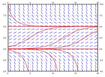
for some positive kk and MM. This equation is commonly used to model population if we know the limiting population MM, that is the maximum sustainable population. The logistic equation leads to less catastrophic predictions on world population than x=kxx'=kx. In the real world there is no such thing as negative population, but we will still consider negative xx for the purposes of the math (see Figure 2\PageIndex{2} for an example).

Slope field over time 0 to 20 and values -5 to 10 with red equilibria at 5 and 0. Solutions above 0 head toward 5, those just below 0 plunge off the bottom, so 5 attracts and 0 repels.
Figure 2\PageIndex{2}: The slope field and some solutions of x=0.1x(5x)x'=0.1x(5-x).

Note two critical points, x=0x = 0 and x=5x = 5. The critical point at x=5x = 5. is stable. On the other hand the critical point at x=0x = 0. is unstable.

It is not really necessary to find the exact solutions to talk about the long term behavior of the solutions. For example, from the above slope field plot, we can easily see that

lim t x ( t ) = { 5 if x ( 0 ) > 0 , 0 if x ( 0 ) = 0 , DNE or if x ( 0 ) < 0 . \lim\limits_{t\to\infty} x(t) = \begin{cases} 5 & \text{if} \, x(0) > 0, \\ 0 & \text{if} \, x(0) = 0, \\ \text{DNE or} -\infty & \text{if} \, x(0) < 0. \end{cases} \nonumber

Where DNE means “does not exist.” From just looking at the slope field we cannot quite decide what happens if x(0)<0x(0) < 0. It could be that the solution does not exist for tt all the way to \infty. Think of the equation x=x2x' = x^2, we have seen that it only exists for some finite period of time. Same can happen here. In our example equation above it will actually turn out that the solution does not exist for all time, but to see that we would have to solve the equation. In any case, the solution does go to - \infty, but it may get there rather quickly.

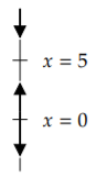
If we are interested only in the long term behavior of the solution, we would be doing unnecessary work if we solved the equation exactly. We could draw the slope field, but it is easier to just look at the phase diagram or phase portrait, which is a simple way to visualize the behavior of autonomous equations. In this case there is one dependent variable xx. We draw the xx-axis, we mark all the critical points, and then we draw arrows in between. Since xx is the dependent variable we draw the axis vertically, as it appears in the slope field diagrams above. If f(x)>0f(x) > 0, we draw an up arrow. If f(x)<0f(x) < 0, we draw a down arrow. To figure this out, we could just plug in some xx between the critical points, f(x)f(x) will have the same sign at all xx between two critical points as long f(x)f(x) is continuous. For example, f(6)=0.6<0f(6) = -0.6 < 0, so f(x)<0f(x) < 0 for x>5x > 5, and the arrow above x=5x=5 is a down arrow. Next, f(1)=0.4>0f(1) = 0.4 > 0, so f(x)>0f(x) > 0 whenever 0<x<50 < x < 5, and the arrow points up. Finally, f(1)=0.6<0f(-1) = -0.6 < 0 so f(x)<0f(x) < 0 when x<0x < 0, and the arrow points down.

Diagram of a vertical phase line with critical points at x = 5 and x = 0. Arrows on both sides of 5 point toward it and the arrow below 0 points away, so 5 is stable and 0 unstable.
Figure 3\PageIndex{3}

Armed with the phase diagram, it is easy to sketch the solutions approximately: As time tt moves from left to right, the graph of a solution goes up if the arrow is up, and it goes down if the arrow is down.

Since any mathematical model we cook up will only be an approximation to the real world, unstable points are generally bad news.

Let us think about the logistic equation with harvesting. Suppose an alien race really likes to eat humans. They keep a planet with humans on it and harvest the humans at a rate of hh million humans per year. Supposexx is the number of humans in millions on the planet and tt is time in years. Let MM be the limiting population when no harvesting is done and k>0k>0 is some constant depending on how fast humans multiply. Our equation becomes

d x d t = k x ( M x ) h \dfrac{dx}{dt} = kx(M-x)-h \nonumber

We expand the right hand side and solve for critical points

d x d t = k x 2 + k M x h \dfrac{dx}{dt} = -kx^2+kMx-h \nonumber

Solving for the critical points AA and BB from the quadratic equations:

A = k M + ( k M ) 2 4 h k 2 k , B = k M ( k M ) 2 4 h k 2 k A= \dfrac{kM + \sqrt{(kM)^2-4hk}}{2k},\quad B= \dfrac{kM - \sqrt{(kM)^2-4hk}}{2k} \nonumber

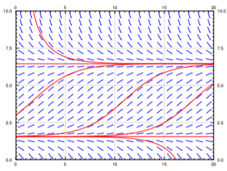
For example, let M=8M=8 and k=0.1k=0.1. When h=1h=1, then AA and BB are distinct and positive. The slope field we get is in Figure 5\PageIndex{5}. As long as the population starts above BB, which is approximately 1.55 million, then the population will not die out. It will in fact tend towards A6.45A \approx 6.45 million. If ever some catastrophe happens and the population drops below BB, humans will die out, and the fast food restaurant serving them will go out of business.
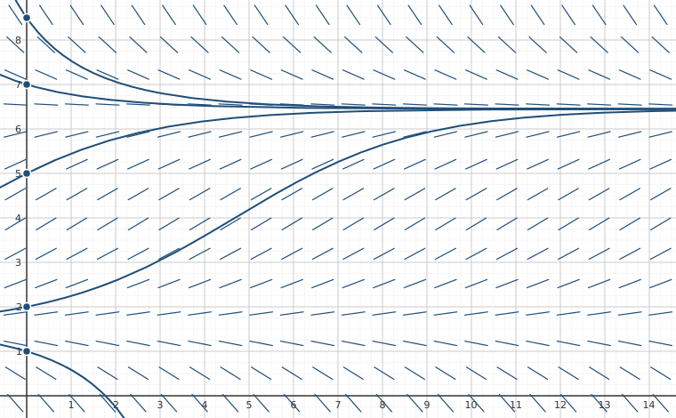
Interactive figureHarvesting slope field for x′ = 0.1x(8 − x) − h, with h on a sliderDrag the Harvest rate h slider from 0 to 2.5.
Short slopes fill the frame, time running left to right and population upward, lying flat along two horizontal levels and tilting toward the upper one from both sides while pointing downward below the lower one. Four of the five solution curves bend into that upper level from above and below; the one starting under the lower level falls away to nothing. Raising the harvest rate drives the two levels together until they merge and vanish, after which every curve plunges to zero however high it starts. Adjustable parameter: Harvest rate h (h) = 1 million/yr. Viewing window: x from -0.6 to 14.6, y from -0.5 to 8.9.
XYZ Graph · viewer build 5edf91b
Figures 5, 6 and 7 are three screenshots of one equation, x′ = 0.1x(8 − x) − h, at three harvest rates; this is all of them at once, with time along the horizontal axis and population up the vertical. Drag h up from 1 and watch the critical points A = 4 + √(16 − 10h) and B = 4 − √(16 − 10h) slide toward each other, collide at h = 1.6 where A = B = 4, then vanish — past which every curve in the frame plummets to zero no matter how well stocked the planet starts.
Slope field over time 0 to 20 and population 0 to 10 with red equilibria at about 6.4 and 1.6. Solutions above the lower line climb or fall toward 6.4; one just below it drops to zero, so 6.4 attracts and 1.6 repels.
Figure 5\PageIndex{5}: Slope field and some solutions of x=0.1x(8x)1x'=0.1x(8-x)-1.

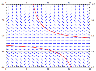
When h=1.6h=1.6, then A=B=4A=B=4 and there is only one critical point and it is unstable. When the population starts above 4 million it will tend towards 4 million. If it ever drops below 4 million, humans will die out on the planet. This scenario is not one that we (as the human fast food proprietor) want to be in. A small perturbation of the equilibrium state and we are out of business; there is no room for error (see Figure 6\PageIndex{6}).

Slope field over time 0 to 20 and population 0 to 10, flat only along the red line at 4. A solution from above eases toward 4, while one starting near 3.5 plummets to zero at about time 15.5.
Figure 6\PageIndex{6}: The slope field and some solutions of x=0.1x(8x)1.6x'=0.1x(8-x)-1.6.

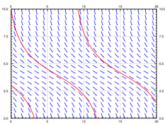
Finally if we are harvesting at 2 million humans per year, there are no critical points. The population will always plummet towards zero, no matter how well stocked the planet starts (see Figure 7\PageIndex{7}).

Slope field over time 0 to 20 and population 0 to 10 with every segment sloping downward, so no equilibrium. Three red solutions fall monotonically to zero, horizontal shifts of one another.
Figure 7\PageIndex{7}: Slope field and some solutions of x=0.1x(8x)2x' = 0.1x(8-x)-2.

Footnotes

[1] Unstable points with one of the arrows pointing towards the critical point are sometimes called semistable.

References

  1. Paul W. Berg and James L. McGregor, Elementary Partial Differential Equations, Holden-Day, San Francisco, CA, 1966.
  2. William E. Boyce, Richard C. DiPrima, Elementary Differential Equations and Boundary Value Problems, 9th edition, John Wiley & Sons Inc., New York, NY, 2008.
  3. C.H. Edwards and D.E. Penney, Differential Equations and Boundary Value Problems: Computing and Modeling, 4th edition, Prentice Hall, 2008.
  4. Stanley J. Farlow, An Introduction to Differential Equations and Their Applications, McGraw-Hill, Inc., Princeton, NJ, 1994. (Published also by Dover Publications, 2006.)
  5. E.L. Ince, Ordinary Differential Equations, Dover Publications, Inc., New York, NY, 1956.

Adapted from Differential Equations for Engineers by Jiří Lebl (https://www.jirka.org/diffyqs/), © Jiří Lebl, licensed under CC BY-SA 4.0. Changes were made. License: CC-BY-SA-4.0.

These eBooks are a prerelease and are not yet certified conformant with WCAG 2.1 AA or ADA Title II. Every page is built against an automated accessibility gate, and the published editions will meet ADA Title II requirements when they release in late September 2026. If something is unusable, please tell us.