1.2 Slope fields

The general first order equation we are studying looks like

$y^{'} = f (x, y)$

In general, we cannot simply solve these kinds of equations explicitly. It would be nice if we could at least figure out the shape and behavior of the solutions, or if we could find approximate solutions. At this point it may be good to first try the Lab I and/or Project I from the IODE website.

Slope fields

The equation $y^{'} = f (x, y)$ gives you a slope at each point in the $(x, y)$ -plane. And this is the slope a solution $y (x)$ would have at $x$ if its value was $y$ . In other words, $f (x, y)$ is the slope of a solution whose graph runs through the point $(x, y)$ . At a point $(x, y)$ , we plot a short line with the slope $f (x, y)$ . For example, if $f (x, y) = x y$ , then at point $open parenthesis 2, 1.5 close parenthesis$ we draw a short line of slope $x y = 2 \times 1.5 = 3$ . So, if $y (x)$ is a solution and $y open parenthesis 2 close parenthesis equals 1.5$ , then the equation mandates that $y prime open parenthesis 2 close parenthesis equals 3$ . See Figure $1$ .

Diagram of an empty grid from -3 to 3 in both directions with one short blue segment at x = 2, y = 1.5, tilted steeply up to the right to mark the slope at that single point. — Figure $1$ : The slope $y^{'} = x y$ at $open parenthesis 2, 1.5 close parenthesis$ .

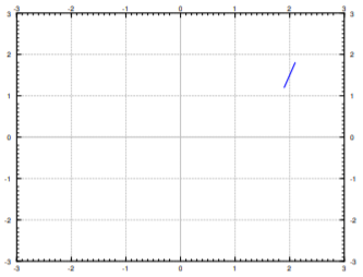
To get an idea of how solutions behave, we draw such lines at lots of points in the plane, not just the point $open parenthesis 2, 1.5 close parenthesis$ . We would ideally want to see the slope at every point, but that is just not possible. Usually we pick a grid of points fine enough so that it shows the behavior, but not too fine so that we can still recognize the individual lines. We call this picture the slope field of the equation. See Example 2 for the slope field of the equation $y^{'} = x y$ . Usually in practice, one does not do this by hand, but has a computer do the drawing.

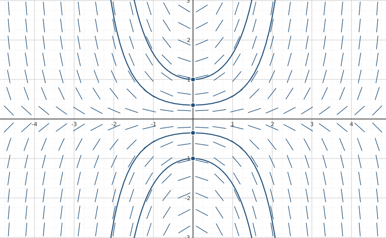
Function graph showing the slope field of the differential equation dy/dx = x*y, drawn from 308 sample slopes, and 4 solution curves through (0, 1), (0, 0.35), (0, -0.35) and (0, -1). Viewing window: x from -4.87 to 4.87, y from -3.01 to 3.01. — The slope field of y′ = xy, the equation this section works through. Explore it to drag the viewing window, or open it in XYZ Graph to add your own initial conditions and watch the solution curve follow the slopes.

Suppose we are given a specific initial condition $y open parenthesis x sub 0 close parenthesis equals y sub 0$ . A solution, that is, the graph of the solution, would be a curve that follows the slopes we drew. For a few sample solutions, see Figure $3$ . It is easy to roughly sketch (or at least imagine) possible solutions in the slope field, just from looking at the slope field itself. You simply sketch a line that roughly fits the little line segments and goes through your initial condition.

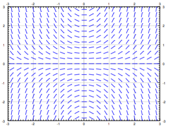
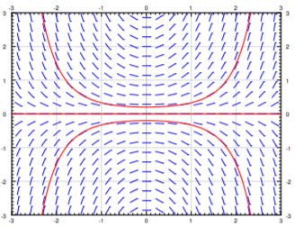
Slope field over x and y from -3 to 3, symmetric about the origin: the dashes lie flat along both axes and steepen with distance from them, standing nearly vertical at the corners. — Figure $3$ : Slope field of $y^{'} = x y$ .

Slope field over x and y from -3 to 3 with three red solutions: the line y = 0 and two curves mirroring it, with turning points at 0.2 and -0.2, that bend sharply away near x = 2.35. — Figure $3$ : Slope field of $y^{'} = x y$ with a graph of solutions satisfying $y open parenthesis 0 close parenthesis equals 0.2$ , $y open parenthesis 0 close parenthesis equals 0$ , and $y (0) = - 0.2$ .

By looking at the slope field we get a lot of information about the behavior of solutions without having to solve the equation. For example, in Figure $3$ we see what the solutions do when the initial conditions are $y open parenthesis 0 close parenthesis greater than 0$ , $y open parenthesis 0 close parenthesis equals 0$ and $y open parenthesis 0 close parenthesis less than 0$ . A small change in the initial condition causes quite different behavior. We see this behavior just from the slope field and imagining what solutions ought to do.

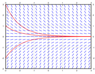
We see a different behavior for the equation $y^{'} = - y$ . The slope field and a few solutions is in see Figure $4$ . If we think of moving from left to right (perhaps $x$ is time and time is usually increasing), then we see that no matter what $y open parenthesis 0 close parenthesis$ is, all solutions tend to zero as $x$ tends to infinity. Again that behavior is clear from simply looking at the slope field itself.

Slope field over x and y from -3 to 3 whose dashes all lean back toward y = 0. Three red solutions entering at y = 3, 1 and -2 merge with the line y = 0 by about x = 1. — Figure $4$ : Slope field of $y^{'} = - y$ with a graph of a few solutions.

Existence and uniqueness

We wish to ask two fundamental questions about the problem

$y^{'} = f (x, y), y (x_{0}) = y_{0}$

Does a solution exist?
Is the solution unique (if it exists)?

What do you think is the answer? The answer seems to be yes to both does it not? Well, pretty much. But there are cases when the answer to either question can be no.

Since generally the equations we encounter in applications come from real life situations, it seems logical that a solution always exists. It also has to be unique if we believe our universe is deterministic. If the solution does not exist, or if it is not unique, we have probably not devised the correct model. Hence, it is good to know when things go wrong and why.

Example 1

Attempt to solve

$y^{'} = \frac{1}{x}, y (0) = 0 .$

Show solution

Integrate to find the general solution $y = \ln | x | + C$ . Note that the solution does not exist at $x equals 0$ . See Figure $5$ on the following page. The equation may have been written as the seemingly harmless $x y prime equals 1$ .

Figure

5

: Slope field of

y^{'} = \frac{1}{x} .

Example 2

Solve:

$y^{'} = 2 \sqrt{| y |}, y (0) = 0 .$

Show solution

Figure

6

: Slope field of

y^{'} = 2 \sqrt{| y |}

with two solutions satisfying

y open parenthesis 0 close parenthesis equals 0.

Note that $y equals 0$ is a solution. But another solution is the function

$y (x) = {\begin{matrix} x^{2} & i f x \geq 0 \\ - x^{2} & i f x < 0 \end{matrix}$

It is hard to tell by staring at the slope field that the solution is not unique. Is there any hope? Of course there is. We have the following theorem, known as Picard’s theorem.to the power 1

Note

Picard’s theorem on existence and uniqueness

If $f (x, y)$ is continuous (as a function of two variables) and $\frac{\partial f}{\partial y}$ exists and is continuous near some $open parenthesis x sub 0, y sub 0 close parenthesis$ , then a solution to

$y^{'} = f (x, y), y (x_{0}) = y_{0}$

exists (at least for $x$ in some small interval) and is unique.

Note that the problems $y^{'} = \frac{1}{x}$ , $y open parenthesis 0 close parenthesis equals 0$ and $y^{'} = 2 \sqrt{| y |}$ , $y open parenthesis 0 close parenthesis equals 0$ do not satisfy the hypothesis of the theorem. Even if we can use the theorem, we ought to be careful about this existence business. It is quite possible that the solution only exists for a short while.

Example 3

For some constant $A$ , solve:

$y^{'} = y^{2} y (0) = A$

Show solution

We know how to solve this equation. First assume that $A not equal to 0$ , so $y$ is not equal to zero at least for some $x$ near 0. So $x^{'} = \frac{1}{y^{2}}$ , so $x = - \frac{1}{y} + C$ , so $y = \frac{1}{C - x}$ . If $y open parenthesis 0 close parenthesis equals A$ , then $C = \frac{1}{A}$ so

$y = \frac{1}{\frac{1}{A} - x}$

If $A equals 0$ , then $y equals 0$ is a solution.

For example, when $A equals 1$ the solution “blows up” at $x equals 1$ . Hence, the solution does not exist for all $x$ even if the equation is nice everywhere. The equation $y^{'} = y^{2}$ certainly looks nice.

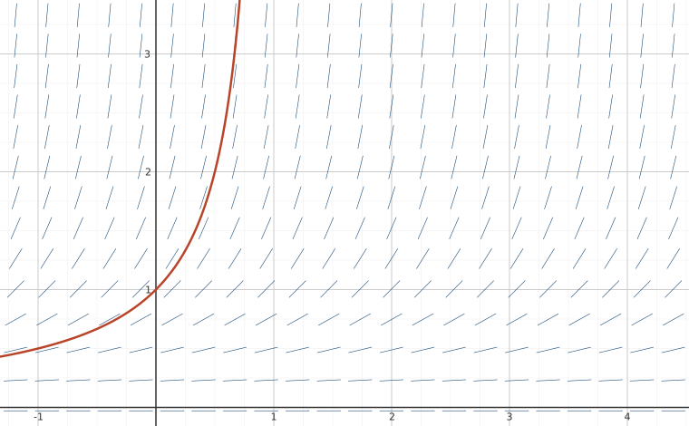
Function graph showing the slope field of the differential equation dy/dx = y^2, drawn from 308 sample slopes and y = 1/(1/a - x). Adjustable parameter: Initial value y(0) = A (a) = 1. Viewing window: x from -1.32 to 4.52, y from -0.16 to 3.46. — The solution of y′ = y², y(0) = A is y = 1/(1/A − x), so it runs into a wall at x = 1/A: how long a solution exists depends on where you start, not on how nice the equation looks. At A = 1 the wall sits at x = 1 — the case worked above. Drag A down to 0.25 and the wall retreats to x = 4; drag it up to 2 and the wall marches in to x = 0.5. The slope field behind the curve shows the mechanism: slopes steepen like y², so the higher the solution climbs the faster it runs away.

For most of this course we will be interested in equations where existence and uniqueness holds, and in fact holds “globally” unlike for the equation $y^{'} = y^{2}$ .

Footnotes

[1] Named after the French mathematician Charles Émile Picard (1856 – 1941)

Adapted from Differential Equations for Engineers by Jiří Lebl (Oklahoma State University), hosted on LibreTexts (math.libretexts.org) and licensed under CC BY-SA 4.0. Changes were made. License: CC-BY-SA-4.0.