1.3 Separable Equations

When a differential equation is of the form $y^{'} = f (x)$ , we can just integrate: $y = \int f (x) d x + C$ . Unfortunately this method no longer works for the general form of the equation $y^{'} = f (x, y)$ . Integrating both sides yields

$y = \int f (x, y) d x + C$

Notice the dependence on $y$ in the integral.

Separable equations

Let us suppose that the equation is separable. That is, let us consider

$y^{'} = f (x) g (y),$

for some functions $f (x)$ and $g (y)$ . Let us write the equation in the Leibniz notation

$\frac{d y}{d x} = f (x) g (y)$

Then we rewrite the equation as

$\frac{d y}{g (y)} = f (x) d x$

Now both sides look like something we can integrate. We obtain

$\int \frac{d y}{g (y)} = \int f (x) d x + C$

If we can find closed form expressions for these two integrals, we can, perhaps, solve for $y .$

Example 1

Take the equation

$y^{'} = x y$

First note that $y equals 0$ is a solution, so assume $y not equal to 0$ from now on, so that we can divide by $y$ . Write the equation as $\frac{d y}{d x} = x y,$ then

$\int \frac{d y}{y} = \int x d x + C .$

We compute the antiderivatives to get

$\ln | y | = \frac{x^{2}}{2} + C$

$| y | = e^{\frac{x^{2}}{2} + C} = e^{\frac{x^{2}}{2}} e^{C} = D e^{\frac{x^{2}}{2}}$

where $D greater than 0$ is some constant. Because $y equals 0$ is a solution and because of the absolute value we actually can write:

$y = D e^{\frac{x^{2}}{2}}$

for any number $D$ (including zero or negative).

We check:

$y^{'} = D x e^{\frac{x^{2}}{2}} = x (D e^{\frac{x^{2}}{2}}) = x y$

Yay!

We should be a little bit more careful with this method. You may be worried that we were integrating in two different variables. We seemingly did a different operation to each side. Let us work through this method more rigorously. Take

$\frac{d y}{d x} = f (x) g (y)$

We rewrite the equation as follows. Note that $y = y (x)$ is a function of $x$ and so is $\frac{d y}{d x}!$

$\frac{1}{g (y)} \frac{d y}{d x} = f (x)$

We integrate both sides with respect to $x .$

$\int \frac{1}{g (y)} \frac{d y}{d x} d x = \int f (x) d x + C$

We use the change of variables formula (substitution) on the left hand side:

$\int \frac{1}{g (y)} d y = \int f (x) d x + C$

And we are done.

Implicit solutions

It is clear that we might sometimes get stuck even if we can do the integration. For example, take the separable equation

$y^{'} = \frac{x y}{y^{2} + 1}$

We separate variables,

$\frac{y^{2} + 1}{y} d y = (y + \frac{1}{y}) d y = x d x$

We integrate to get

$\frac{y^{2}}{2} + l n | y | = \frac{x^{2}}{2} + C$

or perhaps the easier looking expression (where $D equals 2 C$ )

$y^{2} + 2 l n | y | = x^{2} + D$

It is not easy to find the solution explicitly as it is hard to solve for $y$ . We, therefore, leave the solution in this form and call it an implicit solution. It is still easy to check that an implicit solution satisfies the differential equation. In this case, we differentiate with respect to $x$ , and remember that $y$ is a function of $x$ , to get

$y^{'} (2 y + \frac{2}{y}) = 2 x$

Multiply both sides by $y$ and divide by $2 open parenthesis y squared plus 1 close parenthesis$ and you will get exactly the differential equation. We leave this computation to the reader.

If you have an implicit solution, and you want to compute values for $y$ , you might have to be tricky. You might get multiple solutions $y$ for each $x$ , so you have to pick one. Sometimes you can graph $x$ as a function of $y$ , and then flip your paper. Sometimes you have to do more.

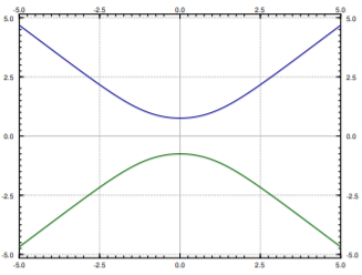
Computers are also good at some of these tricks. More advanced mathematical software usually has some way of plotting solutions to implicit equations. For example, for $C equals 0$ if you plot all the points $(x, y)$ that are solutions to $y^{2} + 2 \ln | y | = x^{2}$ , you find the two curves in Figure $1$ . This is not quite a graph of a function. For each $x$ there are two choices of $y$ . To find a function you would have to pick one of these two curves. You pick the one that satisfies your initial condition if you have one. For example, the top curve satisfies the condition $y open parenthesis 1 close parenthesis equals 1$ . So for each $C$ we really got two solutions. As you can see, computing values from an implicit solution can be somewhat tricky. But sometimes, an implicit solution is the best we can do.

Plot of two mirror-image branches on axes from -5 to 5, a blue one above the horizontal axis bottoming at about 0.7 and a green one below peaking at about -0.7, opening outward like a hyperbola. — Figure $1$ : The implicit solution $y^{2} + 2 \ln | y | = x^{2}$ to $y^{'} = \frac{x y}{y^{2} + 1}$ .

The equation above also has the solution $y equals 0$ . So the general solution is

$y^{2} + 2 \ln | y | = x^{2} + C, and y = 0 .$

These outlying solutions such as

y equals 0

are sometimes called singular solutions.

Example 2

Solve $x^{2} y^{'} = 1 - x^{2} + y^{2} - x^{2} y^{2}$ , $y open parenthesis 1 close parenthesis equals 0.$

Show solution

First factor the right hand side to obtain

$x^{2} y^{'} = (1 - x^{2}) (1 + y^{2})$

Separate variables, integrate, and solve for $y$

$\begin{matrix} \frac{y^{'}}{1 + y^{2}} = \frac{1 - x^{2}}{x^{2}}, \\ \frac{y^{'}}{1 + y^{2}} = \frac{1}{x^{2}} - 1, \\ arctan (y) = - \frac{1}{x^{2}} - x + C, \\ y = \tan (- \frac{1}{x} - x + C) \end{matrix}$

Solve for the initial condition, $0 = \tan (- 2 + C)$ to get $C equals 2$ (or $C = 2 + π$ , or $C = 2 + 2 π$ , etc.). The particular solution we seek is, therefore,

$y = \tan (\frac{- 1}{x} - x + 2) .$

Example 3

Bob made a cup of coffee, and Bob likes to drink coffee only once reaches 60 degrees Celsius and will not burn him. Initially at time $t equals 0$ minutes, Bob measured the temperature and the coffee was 89 degrees Celsius. One minute later, Bob measured the coffee again and it had 85 degrees. The temperature of the room (the ambient temperature) is 22 degrees. When should Bob start drinking?

Show solution

Let $T$ be the temperature of the coffee in degrees Celsius, and let $A$ be the ambient (room) temperature, also in degrees Celsius. states that the rate at which the temperature of the coffee is changing is proportional to the difference between the ambient temperature and the temperature of the coffee. That is,

$\frac{d T}{d t} = k (A - T),$

for some constant $k$ . For our setup $A equals 22$ , $T open parenthesis 0 close parenthesis equals 89$ , $T open parenthesis 1 close parenthesis equals 85$ . We separate variables and integrate (let $C$ and $D$ denote arbitrary constants)

$\begin{matrix} \frac{1}{T - A} \frac{d T}{d t} = - k, \\ \ln (T - A) = - k t + C, (note that T - A > 0) \\ T - A = D e^{- k t}, \\ T = A + D e^{- k t} \end{matrix}$

That is, $T = 22 + D e^{- k t}$ . We plug in the first condition: $89 = T (0) = 22 + D$ , and hence $D equals 67$ . So $T = 22 + 67 e^{- k t}$ . The second condition says $85 = T (1) = 22 + 67 e^{- k}$ . Solving for $k$ we get $k = - \ln \frac{85 - 22}{67} \approx 0.0616$ . Now we solve for the time $t$ that gives us a temperature of 60 degrees. Namely, we solve

$60 = 22 + 67 e^{- 0.0616 t}$

to get

t = - \frac{\ln \frac{60 - 22}{67}}{0.0616} \approx 9.21

minutes. So Bob can begin to drink the coffee at just over 9 minutes from the time Bob made it. That is probably about the amount of time it took us to calculate how long it would take. See Figure

2

Figure

2

: Graphs of the coffee temperature function

T (t)

. On the left, horizontal lines are drawn at temperatures

60

85

, and

89

. Vertical lines are drawn at

t equals 1

and

t equals 9.21

. Notice that the temperature of the coffee hits

85

t equals 1

, and

60

t approximately equals 9.21

. On the right, the graph is over a longer period of time, with a horizontal line at the ambient temperature

22

Adapted from Differential Equations for Engineers by Jiří Lebl (Oklahoma State University), hosted on LibreTexts (math.libretexts.org) and licensed under CC BY-SA 4.0. Changes were made. License: CC-BY-SA-4.0.